Analysis and Control of Antibiotic Dynamic Models

2. Model description

Model 1 Mena, et al. [18]

The model equations are

$\begin{array}{l}\frac{d(sval)}{dt}={\beta }_{s}sval(1-sval-rval)-\alpha sval-{\mu }_{s}sval\\ \frac{d(rval)}{dt}={\beta }_{r}rval(1-sval-rval)+(1-\eta )q\alpha sval-{\mu }_{r}rval\text{ (1)}\end{array}$

sval and rval denote the number of sensitive and resistant bacteria population to antibiotics, respectively. The base values of the parameters are

${\beta }_s=0.4;{\beta }_r=0.1;{\mu }_s=0.2;{\mu }_s=0.5;\alpha =0.1204;q=0.3992;\eta =0.5;$

Model 2 Cen, et al. [17]

$\begin{array}{l}\frac{d(sval)}{dt}=m\mu +\beta sval(xval)-({\tau }_1+{\tau }_2+\gamma +\mu )sval+\sigma \beta c(sval)(rval)\\ \frac{d(rval)}{dt}=\beta xval(1-c)rval-({\tau }_2+\gamma +\mu )rval-\sigma \beta c(sval)(rval)\\ \frac{d(xval)}{dt}=(1-m)\mu +({\tau }_1+{\tau }_2+\gamma +\mu )sval+({\tau }_2+\gamma )rval-\beta sval(xval)\text{ (2)}\\ -\beta xval(1-c)rval-\mu (xval)\end{array}$

The model considers two strains of a bacterial species having two antimicrobial agents. Individuals may have strains of these bacteria that are either sensitive (sval) or resistant (rval) to the first drug, or they may be free of these bacteria (xval). . The base values of the parameters are

$m=0.75;\mu =0.1;\beta =1;{\tau }_1=0.35;{\tau }_2=0.1;\gamma =1/30;\sigma =0.25;c=0.05;$

3. Bifurcation analysis

The MATLAB software MATCONT is used to perform the bifurcation calculations. Bifurcation analysis deals with multiple steady-states and limit cycles. Multiple steady states occur because of the existence of branch and limit points. Hopf bifurcation points cause limit cycles. A commonly used MATLAB program that locates limit points, branch points, and Hopf bifurcation points is MATCONT [19,20]. This program detects Limit Points (LP), Branch Points (BP), and Hopf bifurcation points (H) for an ODE system

$\frac{dx}{dt}=f(x,\alpha )\text{ (3)}$

$x\in R^n$ Let the bifurcation parameter be α. Since the gradient is orthogonal to the tangent vector,

The tangent plane at any point $z=[z_1,z_2,z_3,z_4,\mathrm{....}{z}_{n+1}]$ must satisfy

$Az=0\text{ (4)}$

Where A is

$A=[\partial f/\partial x|\partial f/\partial \alpha ]\text{ (5)}$

where $\partial f/\partial x$ is the Jacobian matrix. For both limit and branch points, the matrix $[\partial f/\partial x]$ must be singular. The n+1th component of the tangent vector $z_{n+1}=0$ for a limit point (LP) and for a branch point (BP) the matrix $\left[\begin{array}{l}A\\ z^T\end{array}\right]$ must be singular. At a Hopf bifurcation point,

$\det (2f_x(x,\alpha )@I_n)=0\text{ (6)}$

@ indicates the bialternate product while I_n is the n-square identity matrix. Hopf bifurcations cause limit cycles and should be eliminated because limit cycles make optimization and control tasks very difficult. More details can be found in Kuznetsov [21,22] and Govaerts [23].

Hopf bifurcations cause unwanted oscillatory behavior and limit cycles. The tanh activation function (where a control value u is replaced by) $(u\tanh u/\epsilon )$ is commonly used in neural nets [24]; Kamalov, et al. [25] and Szandała 2020 [26] and optimal control problems [27] to eliminate spikes in the optimal control profile. Hopf bifurcation points cause oscillatory behavior. Oscillations are similar to spikes, and the results in Sridhar [24] demonstrate that the tanh factor also eliminates the Hopf bifurcation by preventing the occurrence of oscillations. Sridhar [28] explained with several examples how the activation factor involving the tanh function successfully eliminates the limit cycle causing Hopf bifurcation points. This was because the tanh function increases the time period of the oscillatory behavior, which occurs in the form of a limit cycle caused by Hopf bifurcations.

4. Multiobjective Nonlinear Model Predictive Control (MNLMPC)

Flores Tlacuahuaz, et al. [29] developed a Multiobjective Nonlinear Model Predictive Control (MNLMPC) method that is rigorous and does not involve weighting functions or additional constraints. This procedure is used for performing the MNLMPC calculations Here ${\displaystyle \sum _{t_{i=0}}^{t_i=t_f}{q}_j(t_i)}\left(\text{j}=\text{1},\text{ 2}\mathrm{..}\text{n}\right)$ represents the variables that need to be minimized/maximized simultaneously for a problem involving a set of ODE

$\frac{dx}{dt}=F(x,u)\text{ (7)}$

t_f being the final time value, and n the total number of objective variables and .u the control parameter. This MNLMPC procedure first solves the single objective optimal control problem independently optimizing each of the variables ${\displaystyle \sum _{t_{i=0}}^{t_i=t_f}{q}_j(t_i)}$ individually. The minimization/maximization of ${\displaystyle \sum _{t_{i=0}}^{t_i=t_f}{q}_j(t_i)}$ will lead to the values $q_j^{*}$ . Then the optimization problem that will be solved is

$\begin{array}{l}\min ({\displaystyle \sum _{j=1}^n({\displaystyle \sum _{t_{i=0}}^{t_i=t_f}{q}_j(t_i)}-q_j^{*}){)}^2}\text{ (8)}\\ subjectto\frac{dx}{dt}=F(x,u);\end{array}$

This will provide the values of u at various times. The first obtained control value of u is implemented and the rest are discarded. This procedure is repeated until the implemented and the first obtained control values are the same or if the Utopia point where $({\displaystyle \sum _{t_{i=0}}^{t_i=t_f}{q}_j(t_i)}=q_j^{*}\text{for all j})$ is obtained.

Pyomo [30] is used for these calculations. Here, the differential equations are converted to a Nonlinear Program (NLP) using the orthogonal collocation method The NLP is solved using IPOPT [31] and confirmed as a global solution with BARON [32].

The steps of the algorithm are as follows

1. Optimize  ${\displaystyle \sum _{t_{i=0}}^{t_i=t_f}{q}_j(t_i)}$ and obtain  $q_j^{*}$ at various time intervals ti. The subscript i is the index for each time step.
2. Minimize $({\displaystyle \sum _{j=1}^n({\displaystyle \sum _{t_{i=0}}^{t_i=t_f}{q}_j(t_i)}-q_j^{*}){)}^2}$ and get the control values for various times.
3. Implement the first obtained control values
4. Repeat steps 1 to 3 until there is an insignificant difference between the implemented and the first obtained value of the control variables or if the Utopia point is achieved. The Utopia point is when  ${\displaystyle \sum _{t_{i=0}}^{t_i=t_f}{q}_j(t_i)}=q_j^{*}$ for all j.

Sridhar [33] proved that the MNLMPC calculations to converge to the Utopia solution when the bifurcation analysis revealed the presence of limit and branch points. This was done by imposing the singularity condition on the co-state equation [34]. If the minimization of q₁ lead to the value $q_1^{*}$ and the minimization of q₂ lead to the value $q_1^{*}$ The MNLPMC calculations will minimize the function ${(q_1-q_1^{*})}^2+{(q_2-q_2^{*})}^2$ . The multiobjective optimal control problem is

$\min {(q_1-q_1^{*})}^2+{(q_2-q_2^{*})}^{2}subjectto\frac{dx}{dt}=F(x,u)\text{ (9)}$

Differentiating the objective function results in

$\begin{array}{l}\frac{d}{d{x}_i}({(}^{q_1}+{(}^{q_2})=2(q_1-q_1^{*})\frac{d}{d{x}_i}(q_1-q_1^{*})\text{ (10)}\\ +2(q_2-q_2^{*})\frac{d}{d{x}_i}(q_2-q_2^{*})\end{array}$

The Utopia point requires that both $(q_1-q_1^{*})\text{ and }(q_2-q_2^{*})$ are zero. Hence

$\frac{d}{d{x}_i}({(q_1-q_1^{*})}^2+{(q_2-q_2^{*})}^2)=0\text{ (11)}$

the optimal control co-state equation [34] is

$\frac{d}{dt}({\lambda }_i)=-\frac{d}{d{x}_i}({(q_1-q_1^{*})}^2+{(q_2-q_2^{*})}^2)-f_x{\lambda }_i;{\lambda }_i(t_f)=0\text{ (12)}$

λ_i is the Lagrangian multiplier. tf is the final time. The first term in this equation is 0 and hence

$\frac{d}{dt}({\lambda }_i)=-f_x{\lambda }_i;{\lambda }_i(t_f)=0\text{ (13)}$

At a limit or a branch point, for the set of ODE $\frac{dx}{dt}=f(x,u)$ fx is singular. Hence there are two different vectors-values for [λ_i] where $\frac{d}{dt}({\lambda }_i)>0\text{ and }\frac{d}{dt}({\lambda }_i)<0$ . In between there is a vector [λ_i] where $\frac{d}{dt}({\lambda }_i)=0$ . This, coupled with the boundary condition ${\lambda }_i(t_f)=0$ will lead to [λ_i] = 0 This makes the problem an unconstrained optimization problem, and the only solution is the Utopia solution.

5. Results

Model 1

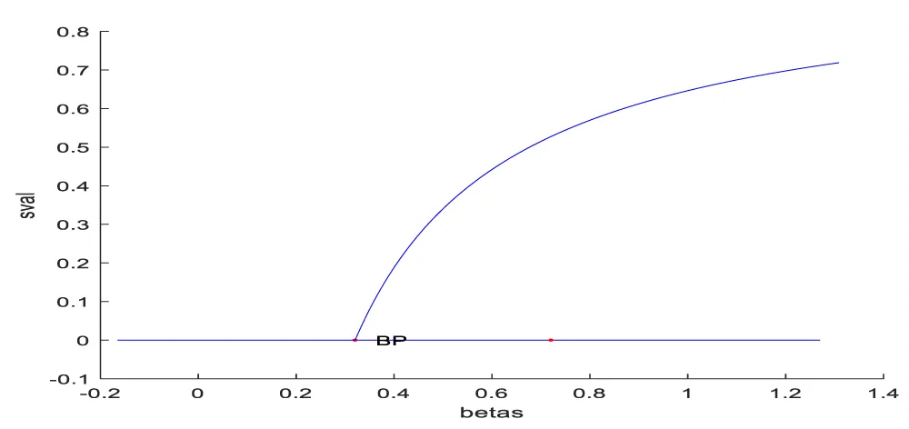
The bifurcation analysis (with βs as the bifurcation parameter) revealed a branch point at $(sval,rval,{\beta }_s)$ values of (0, 0, 0.3204).

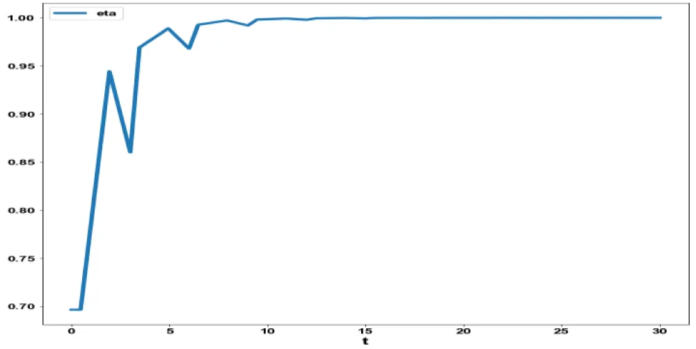
This is shown in Figure 1a. For the MNLMPC calculations, ${\displaystyle \sum _{t_{i=0}}^{t_i=t_f}rval(t_i)},{\displaystyle \sum _{t_{i=0}}^{t_i=t_f}\eta (t_i)}$ were minimized individually and led to values of 0 and 0. η was the control parameter. 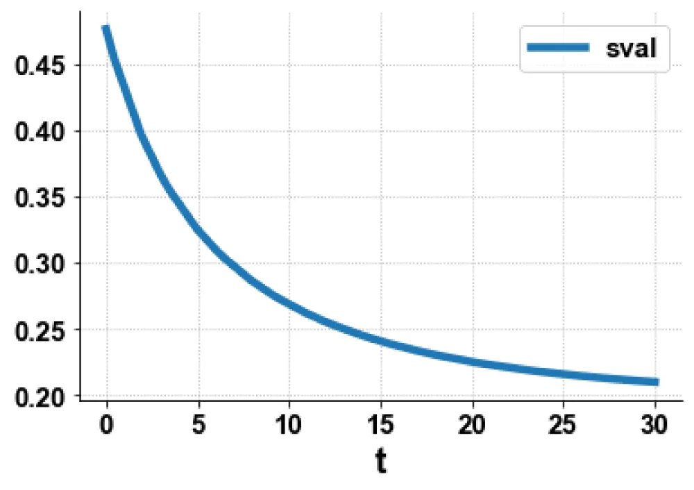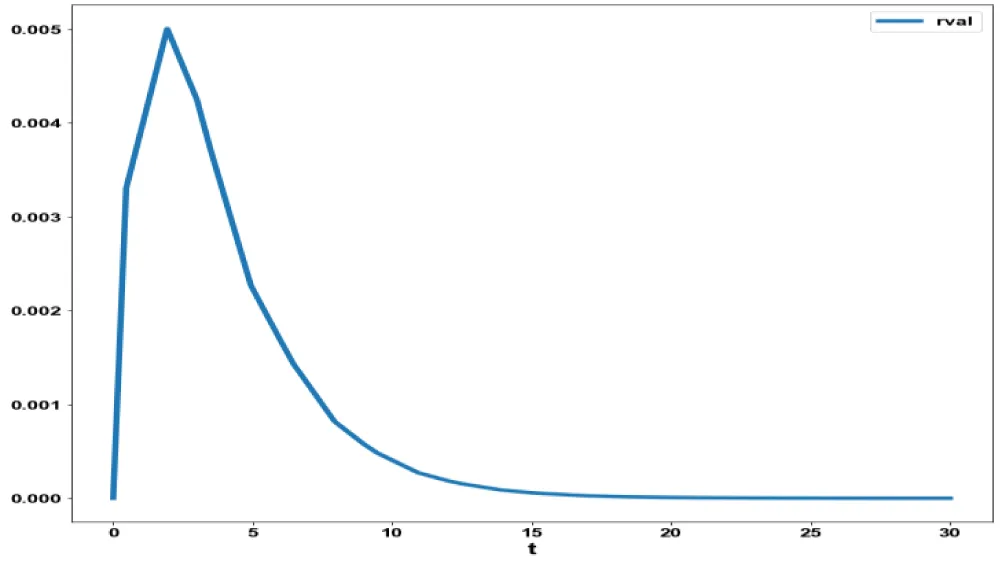The multiobjective optimal control problem will involve the minimization of ${({\displaystyle \sum _{t_{i=0}}^{t_i=t_f}rval(t_i)})}^2+{({\displaystyle \sum _{t_{i=0}}^{t_i=t_f}\eta (t_i)})}^2$ subject to the equations governing Model 1. This led to a value of zero (the Utopia solution). The MNLMPC control value (η) was 0.6963. Figures 1(b-d). show the various MNLMPC profiles.

Figure 1a: Bifurcation analysis of Antibiotic model 1 (indicating branch point).

Figure 1b: MNLMPC model 1 sval vs. t.

Figure 1c: MNLMPC model 1 rval vs. t.

Figure 1d: MNLMPC model 1 eta (n) vs.t.

Model 2

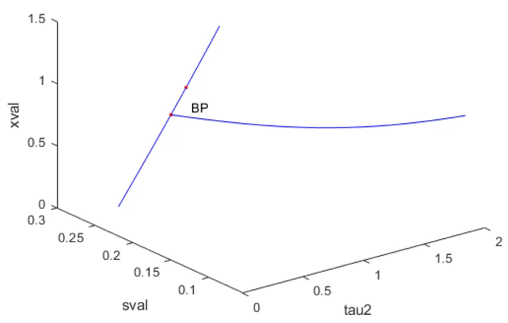
The bifurcation analysis (with τ2 as the bifurcation parameter) revealed a branch point at $(sval,rval,xval,{\tau }_2)$ values of (0.242641, 0, 0.757359, 0.583125). This is shown in Figure 2a.

Figure 2a: Bifurcation analysis of Antibiotic model 2 (indicating branch point).

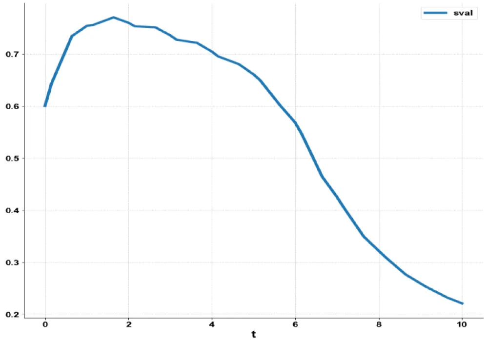
For the MNLMPC calculations, sval(0)=0.6; ${\displaystyle \sum _{t_{i=0}}^{t_i=t_f}rval(t_i)}$ was minimized and ${\displaystyle \sum _{t_{i=0}}^{t_i=t_f}xval(t_i)}$ was maximized leading to values of 0 and 2. 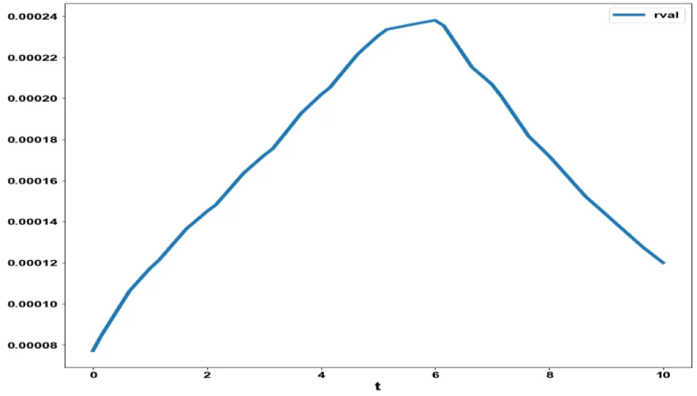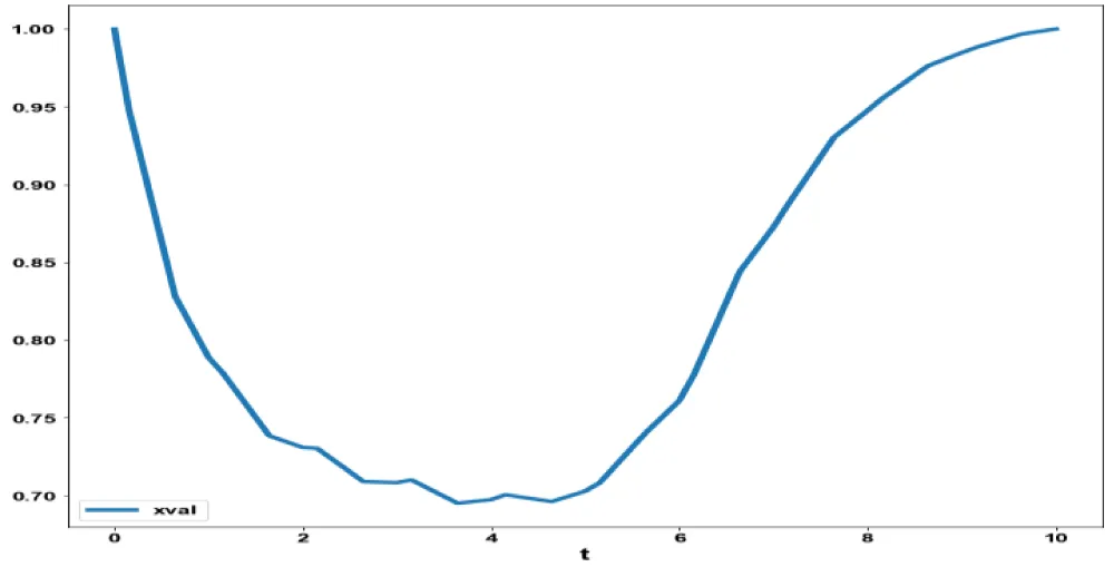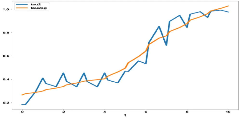The multiobjective optimal control problem will involve the minimization of ${({\displaystyle \sum _{t_{i=0}}^{t_i=t_f}rval(t_i)})}^2+{({\displaystyle \sum _{t_{i=0}}^{t_i=t_f}xval(t_i)-2})}^2$ and resulted in the Utopia point(0). The MNLMPC control value (τ2) was 0.18248. Figures 2(b-d). show the various MNLMPC profiles. The profile of the control variable (τ2) exhibited a lot of noise, which was remedied using the Savitzky-Golay filter. Both the original and the modified profiles are shown in Figure 2e.

Figure 2b: MNLMPC model 2 sval vs. t.

Figure 2c: MNLMPC model 2 rval vs. t.

Figure 2d: MNLMPC model 2 xval vs. t.

Figure 2e: MNLMPC model 2 tau2(τ2) with noise and tau2sg (with Savitzky Golay Filter) vs.t.

6. Discussion of results

Theorem

If one of the functions in a dynamic system is separable into two distinct functions, a branch point singularity will occur in the system.

Proof

Consider a system of equations

$\frac{dx}{dt}=f(x,\alpha )\text{ (14)}$

$x\in R^n$ . Defining the matrix A as

$A=\left[\begin{array}{l}\frac{\partial f_1}{\partial x_1}\frac{\partial f_1}{\partial x_2}\frac{\partial f_1}{\partial x_3}\frac{\partial f_1}{\partial x_4}\mathrm{..........}\frac{\partial f_1}{\partial x_n}\frac{\partial f_1}{\partial \alpha }\\ \frac{\partial f_2}{\partial x_1}\frac{\partial f_2}{\partial x_2}\frac{\partial f_2}{\partial x_3}\frac{\partial f_2}{\partial x_4}\mathrm{..........}\frac{\partial f_2}{\partial x_n}\frac{\partial f_2}{\partial \alpha }\\ \mathrm{...........................................................}\\ \mathrm{...........................................................}\\ \frac{\partial f_n}{\partial x_1}\frac{\partial f_n}{\partial x_2}\frac{\partial f_n}{\partial x_3}\frac{\partial f_n}{\partial x_4}\mathrm{..........}\frac{\partial f_n}{\partial x_n}\frac{\partial f_n}{\partial \alpha }\end{array}\right]\text{ (15)}$

α is the bifurcation parameter. The matrix A can be written in a compact form as

$A=[\frac{\partial f_p}{\partial x_q}.|\frac{\partial f_p}{\partial \alpha }]\text{ (16)}$

The tangent at any point x; $(z=[z_1,z_2,z_3,z_4,\mathrm{....}{z}_{n+1}])$ must satisfy

$Az=0\text{ (17)}$

The matrix $\left\{\frac{\partial f_p}{\partial x_q}\right\}$ must be singular at both limit and branch points. The n+1th component of the tangent vector $z_{n+1}=0$ at a limit point (LP) and for a branch point (BP) the matrix $B=\left[\begin{array}{l}A\\ z^T\end{array}\right]$ must be singular.

Any tangent at a point y that is defined by $(z=[z_1,z_2,z_3,z_4,\mathrm{....}{z}_{n+1}])$ must satisfy

$Az=0\text{ (18)}$

For a branch point, there must exist two tangents at the singularity. Let the two tangents be z and w. This implies that

$\begin{array}{l}Az=0\text{ (19)}\\ Aw=0\end{array}$

Consider a vector v that is orthogonal to one of the tangents (say z). v can be expressed as a linear combination of z and $\text{w }(v=\alpha z+\beta w).$ Since $Az=Aw=0;Av=0$ and since z and v are orthogonal,

$z^{T}v=0$ . Hence $Bv=\left[\begin{array}{l}A\\ z^T\end{array}\right]v=0$ which implies that B is singular.

Let any of the functions fi are separable into 2 functions φ1, φ2 as

$f_i={\varphi }_1{\varphi }_2\text{ (20)}$

At steady-state $f_i(x,\alpha )=0$ and this will imply that either φ1 = 0 or φ2 = 0 or both φ1 and φ2 must be 0. This implies that two branches φ1 = 0 and φ2 = 0 will meet at a point where both φ1 and 2 are 0.

At this point, the matrix B will be singular as a row in this matrix would be

$[\frac{\partial f_i}{\partial x_k}|\frac{\partial f_i}{\partial \alpha }]\text{ (21)}$

However,

$\begin{array}{l}[\frac{\partial f_i}{\partial x_k}={\varphi }_1(=0)\frac{\partial {\varphi }_2}{\partial x_k}+{\varphi }_2(=0)\frac{\partial {\varphi }_1}{\partial x_k}=0(\forall k=1.,,n)\text{ (22)}\\ \frac{\partial f_i}{\partial \alpha }={\varphi }_1(=0)\frac{\partial {\varphi }_2}{\partial \alpha }+{\varphi }_2(=0)\frac{\partial {\varphi }_1}{\partial \alpha }]=0\end{array}$

This implies that every element in the row $[\frac{\partial f_i}{\partial x_k}|\frac{\partial f_i}{\partial \alpha }]$ would be 0, and hence the matrix B would be singular. The singularity in B implies that there exists a branch point.

Model 1

In the antibiotic model 1, a branch point was located at $(sval,rval,{\beta }_s)$ values of (0, 0, 0.3204). Here, the two distinct functions can be obtained from the first ODE in the antibiotic model 1

$\frac{d(sval)}{dt}={\beta }_{s}sval(1-sval-rval)-\alpha sval-{\mu }_{s}sval\text{ (23)}$

The two distinct functions are

$sval=0\text{ (24)}$

and

${\beta }_s(1-sval-rval)-\alpha -{\mu }_s=0\text{ (25)}$

Substituting sval=0, rval=0, βs = 0.3204, µs = 0.2, α = 0.1204 satisfies both the distict function equations and validates the theorem computationally.

Model 2

In the antibiotic model 1, a branch point was located at $(sval,rval,xval,{\tau }_2)$ values of (0.242641, 0, 0.757359, 0.583125).

Here the two distinct functions can be obtained from the second ODE in model 2

$\frac{d(rval)}{dt}=\beta xval(1-c)rval-({\tau }_2+\gamma +\mu )rval-\sigma \beta c(sval)(rval)\text{ (26)}$

The two distinct functions are

$rval=0\text{ (27)}$

and

$\beta xval(1-c)-({\tau }_2+\gamma +\mu )-\sigma \beta c(sval)=0\text{ (28)}$

Substituting $(sval,rval,xval,{\tau }_2)$ values of (0.242641, 0, 0.757359, 0.583125) and

$\mu =0.1;\beta =1;\gamma =1/30;\sigma =0.25;c=0.05;$ satisfies both equations, validating the theorem.

Additionally, the MNLMPC calculations in both models converge to the Utopia solution, justifying the analysis of Sridhar [33].

7. Conclusion

Bifurcation analysis and multiobjective nonlinear control (MNLMPC) studies in two antibiotic models. The bifurcation analysis revealed the existence and branch points in both models. The branch points (which cause multiple steady-state solutions from a singular point) are very beneficial because they enable the Multiobjective nonlinear model predictive control calculations to converge to the Utopia point (the best possible solution) in the models. It is proved (with computational validation) that the branch points were caused because of the existence of two distinct separable functions in one of the equations in each dynamic model. A theorem was developed to demonstrate this fact for any dynamic model. A combination of bifurcation analysis and Multiobjective Nonlinear Model Predictive Control (MNLMPC) for dynamic models involving antibiotics is the main contribution of this paper.

Data availability statement

All data used is presented in the paper