Dynamic Analysis and Optimal Control of Probiotic Dynamic Models

Probiotic therapy involves using live microorganisms, primarily bacteria and yeasts, to improve or restore the balance of beneficial bacteria in the body, particularly in the gut. These microorganisms, when administered in adequate amounts, can offer health benefits to the host. Probiotic therapy is used for various conditions, including diarrhea, irritable bowel syndrome (IBS), and even to support immune function. The dynamics of probiotic therapy are extremely nonlinear. Bifurcation analysis is a powerful mathematical tool used to deal with the nonlinear dynamics of any process. Several factors must be considered, and multiple objectives must be met simultaneously. Bifurcation analysis and multi-objective nonlinear model predictive control (MNLMPC) calculations are performed on two dynamic models of probiotic therapy. The MATLAB program MATCONT was used to perform the bifurcation analysis. The MNLMPC calculations were performed using the optimization language PYOMO in conjunction with the state-of-the-art global optimization solvers IPOPT and BARON. The bifurcation analysis revealed the existence of branch points in both models. The branch points (which cause multiple steady-state solutions from a singular point) are very beneficial because they enable the Multiobjective nonlinear model predictive control calculations to converge to the Utopia point (the best possible solution) in the models. It is proven (with computational validation) that the branch points were caused because of the existence of two distinct separable functions in one of the equations in each dynamic model. A theorem was developed to demonstrate this fact for any dynamic model.

Background

A significant amount of work involving probiotic therapy has been conducted over the last century. This is because it was discovered that using live microorganisms, primarily bacteria and yeasts, can improve or restore the balance of beneficial bacteria in the body, and immunity can be improved by these microorganisms. Mattar, et al. [1] studied the effect of probiotics on enterocyte bacterial translocation in vitro. Dani, et al. [2] studied the use of Probiotics feeding in the prevention of urinary tract infections. Millar, et al. [3] investigated the use of probiotics for preterm infants. Bin-Nun, et al. [4] studied the use of oral probiotics to prevent necrotizing enterocolitis. Land, et al. [5] showed that Lactobacillus sepsis was associated with probiotic therapy. Szajewska, et al. [6] investigated the efficacy of probiotics in gastrointestinal diseases in children. Hammerman and Kaplan [7] discussed the connection between probiotics and neonatal intestinal infection. Barclay, et al. [8] reviewed the use of probiotics for necrotizing enterocolitis. AlFaleh, et al. [9] studied the use of probiotics for the prevention of necrotizing enterocolitis in preterm infants. Lin, et al. [10] showed that oral probiotics prevent necrotizing enterocolitis in very low birth weight preterm infants. Claud and Walker [11] studied bacterial colonization, probiotics, and necrotizing enterocolitis. Arciero, et al. [12] developed a mathematical model to analyze the Role of Probiotics and Inflammation in Necrotizing Enterocolitis. Zhang, et al. [13] investigated the impacts of gut bacteria on human health and diseases. Ahmed and Jawad [14] performed a bifurcation analysis of the role of good and bad bacteria in the decomposing toxins in the intestine with the impact of antibiotics and probiotics supplements. This work aims to perform bifurcation analysis and multiobjective nonlinear control (MNLMPC) studies in two models involving probiotics, which are discussed in Arciero, et al. [12] (model 1), and Ahmed and Jawad [14](model 2). The paper is organized as follows. First, the model equations are presented, followed by a discussion of the numerical techniques involving bifurcation analysis and multiobjective nonlinear model predictive control (MNLMPC). The results are then presented, followed by the discussion and conclusions.

Model description

Probiotic Model 1Arciero, et al. [12]

The model equations are

$\begin{array}{l}\frac{d(bl)}{dt}=r_1(bl)\left(1-\frac{\left(bl+\left({\alpha }_1*bpbl\right)\right)}{k1}\right)-eps(bl)\\ \frac{d(bpbl)}{dt}=r_2(bpbl)\left(1-\frac{\left(bpbl+\left({\alpha }_2*bl\right)\right)}{k2}\right)-eps(k)bpbl\\ \frac{d(eps)}{dt}=\left(\frac{\left(eps0-eps\right)}{\tau }\right)+\left(\frac{f\left(epsmax-eps\right)mv}{1+\left(c(bpbl)\right)}\right)\\ \frac{d(b)}{dt}=(bl+k(bpbl))eps-tpar+\left(\frac{bl}{\left(bl+\left(k*bpbl\right)\right)}\right)-\left(k5mv(b)\right)\\ \frac{d(bpb)}{dt}=(bl+k(bpbl))eps-tpar+\left(\frac{k(bpbl)}{\left(bl+\left(k*bpbl\right)\right)}\right)-\left(k6mv(bpb)\right)\text{ (1)}\\ \frac{d(mv)}{dt}={\nu }_1\frac{c1(b)+c2(bpb)}{{\nu }_2+c1(b)+c2(bpb)}-\left(\mu (mv)\right);\end{array}$

Here, bl represents the pathogenic bacteria in the intestinal lumen, bpbl represents the Probiotic bacteria in the intestinal lumen, ε the permeability of the intestinal wall to bacteria, b is the pathogenic bacteria in the blood/tissue, bpb represents the probiotic bacteria in the blood/tissue, and mv represents the activated inflammatory cells.

The parameter values are

$\begin{array}{l}{r}_1=0.55;{\alpha }_1=0.6;{\alpha }_2=0.4;k1=20;k2=10;\epsilon 0=0.1;\epsilon max=0.21;\\ \tau =24;f=0.5;c=0.35;k=0.5;\mu =0.05;k5=25;k6=25;{\nu }_1=0.08;\\ {\nu }_2=0.12;c1=0.1;c2=0.01;tpar=1.5\end{array}$

R2 was used as the bifurcation parameter and the control value.

Probiotic model 2Ahmed and Jawad [14]

The dynamic model equations are

$\begin{array}{l}\frac{d(b_1)}{dt}=(1-\left(\frac{b_1+\left({\alpha }_1{b}_2\right)}{k}\right)r_1(b_1)+\left({\beta }_0{b}_1\right)-\left(\left({\beta }_1+{\gamma }_1\right)(a)b_1\right)-\left({\mu }_1{b}_1\right)\hfill \\ \frac{d(b_2)}{dt}=(1-\left(\frac{b_2+\left({\alpha }_2{b}_1\right)}{k}\right)r_2(b_2)-a{b}_2{\gamma }_2-b_2{\gamma }_0-{\mu }_2{b}_2\hfill \\ \begin{array}{l}\frac{d(c)}{dt}=(c0-c)d+q_1{b}_{2}c-q_2{b}_{1}c\\ \frac{d(a)}{dt}=\omega -{\mu }_{0}a\end{array}\hfill \end{array}\text{ (2)}$

(b1,b2,c,a) represent the good bacteria, the bad bacteria, the non-decomposing toxins in the large intestine, and the concentration of dissolved antibiotics. The base parameter values are

$\begin{array}{l}{r}_2=0.4;k=40;{\alpha }_1=0.1;{\alpha }_2=0.1;{\delta }_1=0.16;{\delta }_2=0.16;\\ {\beta }_0=0.14;{\beta }_1=0.016;{\mu }_1=0.5;{\mu }_2=0.5;{\gamma }_1=0.018;{\gamma }_2=0.017;\\ {\gamma }_0=0.18;d=0.32;c_0=4;q_1=0.012;q_2=0.014;\omega =0.6;{\mu }_0=0.118\end{array}$

r1 was used as the bifurcation parameter and control value.

Bifurcation analysis

The MATLAB software MATCONT is used to perform the bifurcation calculations. Bifurcation analysis deals with multiple steady states and limit cycles. Multiple steady states occur because of the existence of branch and limit points. Hopf bifurcation points cause limit cycles. A commonly used MATLAB program that locates limit points, branch points, and Hopf bifurcation points is MATCONT [15,16]. This program detects Limit points (LP), branch points (BP), and Hopf bifurcation points (H) for an ODE system

$\frac{dx}{dt}=f(x,\alpha )\text{ (3)}$

$x\in R^n$ Let the bifurcation parameter be α. Since the gradient is orthogonal to the tangent vector,

The tangent plane at any point must satisfy.

$Az=0\text{ (4)}$

Where A is

$A=[\partial f/\partial x|\partial f/\partial \alpha ]\text{ (5)}$

Where is the Jacobian matrix? For both limit and branch points, the matrix must be singular. The n+1th component of the tangent vector Z_n+1 = 0 for a limit point (LP), and a branch point (BP), the matrix must be singular. At a Hopf bifurcation point,

$\det (2f_x(x,\alpha )@I_n)=0\text{ (6)}$

@ indicates the bialternate product while is the n-square identity matrix. Hopf bifurcations cause limit cycles and should be eliminated because limit cycles make optimization and control tasks very difficult. More details can be found in Kuznetsov [17,18] and Govaerts [19].

Hopf bifurcations cause unwanted oscillatory behavior and limit cycles. The tanh activation function (where a control value u is replaced by ) $(u\tanh u/\epsilon )$ is commonly used in neural nets [20-23] to eliminate spikes in the optimal control profile. Hopf bifurcation points cause oscillatory behavior. Oscillations are similar to spikes, and the results in Sridhar [24] demonstrate that the tanh factor also eliminates the Hopf bifurcation by preventing the occurrence of oscillations. Sridhar [24] explained with several examples how the activation factor involving the tanh function successfully eliminates the limit cycle causing Hopf bifurcation points. This was because the tanh function increases the period of the oscillatory behavior, which occurs in the form of a limit cycle caused by Hopf bifurcations.

Multiobjective Nonlinear Model Predictive Control (MNLMPC)

Flores Tlacuahuaz, et al. [25] developed a multiobjective nonlinear model predictive control (MNLMPC) method that is rigorous and does not involve weighting functions or additional constraints. This procedure is used for performing the MNLMPC calculations. Here ${\displaystyle \sum _{t_{i=0}}^{t_i=t_f}{q}_j(t_i)}$ (j = 1, 2..n) represents the variables that need to be minimized/maximized simultaneously for a problem involving a set of ODEs.

$\frac{dx}{dt}=F(x,u)\text{ (7)}$

t_f Being the final time value, n is the total number of objective variables, and u is the control parameter. This MNLMPC procedure first solves the single-objective optimal control problem, independently optimizing each of the variables. The minimization/maximization of will lead to the values. Then the optimization problem that will be solved is

$\begin{array}{l}\min ({\displaystyle \sum _{j=1}^n({\displaystyle \sum _{t_{i=0}}^{t_i=t_f}{q}_j(t_i)}-q_j^{*}){)}^2}\text{ (8)}\\ subjectto\frac{dx}{dt}=F(x,u);\end{array}$

This will provide the values of u at various times. The first obtained control value of u is implemented, and the rest are discarded. This procedure is repeated until the implemented and the first obtained control values are the same, or if the Utopia point where ( ${\displaystyle \sum _{t_{i=0}}^{t_i=t_f}{q}_j(t_i)}=q_j^{*}$ for all j) is obtained.

Pyomo [26] is used for these calculations. Here, the differential equations are converted to a Nonlinear Program (NLP) using the orthogonal collocation method. The NLP is solved using IPOPT [27] and confirmed as a global solution with BARON [28].

The steps of the algorithm are as follows.

1. Optimize and obtain at various time intervals, t_i. The subscript i is the index for each time step.
2. Minimize  $({\displaystyle \sum _{j=1}^n({\displaystyle \sum _{t_{i=0}}^{t_i=t_f}{q}_j(t_i)}-q_j^{*}){)}^2}$ and get the control values for various times.
3. Implement the first obtained control values.
4. Repeat steps 1 to 3 until there is an insignificant difference between the implemented and the first obtained value of the control variables or if the Utopia point is achieved. The Utopia point is when for all j.

Sridhar [29] proved that the MNLMPC calculations converge to the Utopia solution when the bifurcation analysis revealed the presence of limit and branch points. This was done by imposing the singularity condition on the co-state equation [30]. If the minimization of lead to the value and the minimization of lead to the value, the MNLPMC calculations will minimize the function. The multiobjective optimal control problem is

$\begin{array}{l}\min {(}^{q_1}+{(}^{q_2}subjectto\frac{dx}{dt}=F(x,u)\text{ (9)}\\ \end{array}$

Differentiating the objective function results in

$\frac{d}{d{x}_i}({(q_1-q_1^{*})}^2+{(q_2-q_2^{*})}^2)=2(q_1-q_1^{*})\frac{d}{d{x}_i}(q_1-q_1^{*})+2(q_2-q_2^{*})\frac{d}{d{x}_i}(q_2-q_2^{*})\text{ (10)}$

The Utopia point requires that both are zero. Hence

$\frac{d}{d{x}_i}({(q_1-q_1^{*})}^2+{(q_2-q_2^{*})}^2)=0\text{ (11)}$

The optimal control co-state equation [30] is

$\frac{d}{dt}({\lambda }_i)=-\frac{d}{d{x}_i}({(q_1-q_1^{*})}^2+{(q_2-q_2^{*})}^2)-f_x{\lambda }_i;{\lambda }_i(t_f)=0\text{ (12)}$

λi Is the Lagrangian multiplier. tf This is the final time. The first term in this equation is 0, and hence.

$\frac{d}{dt}({\lambda }_i)=-f_x{\lambda }_i;{\lambda }_i(t_f)=0\text{ (13)}$

At a limit or a branch point, the set of ODE $\frac{dx}{dt}=f(x,u)$ f_x is singular. Hence, there are two different vector values for where and. In between, there is a vector where. This, coupled with the boundary condition, will lead to. This makes the problem an unconstrained optimization problem, and the only solution is the Utopia solution.

Results

Probiotic model 1

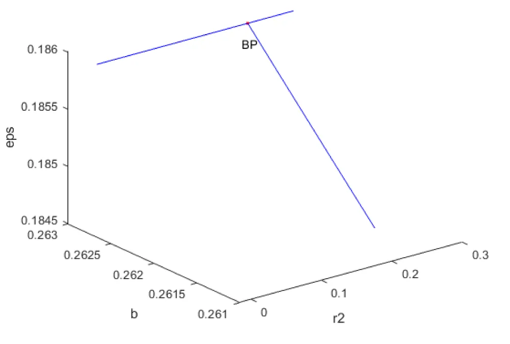
When r2 was used as the urcation parameter, a branch point was located at

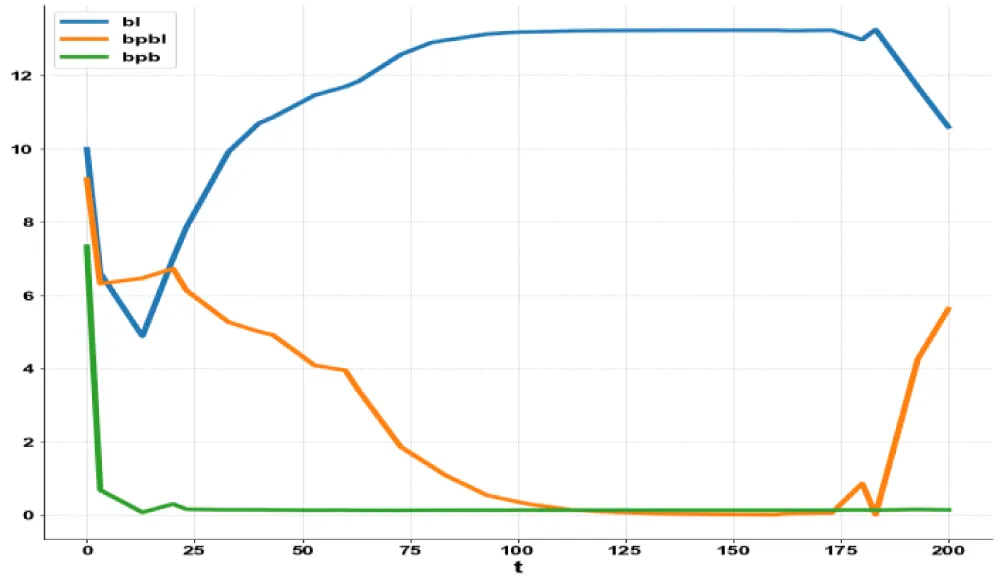
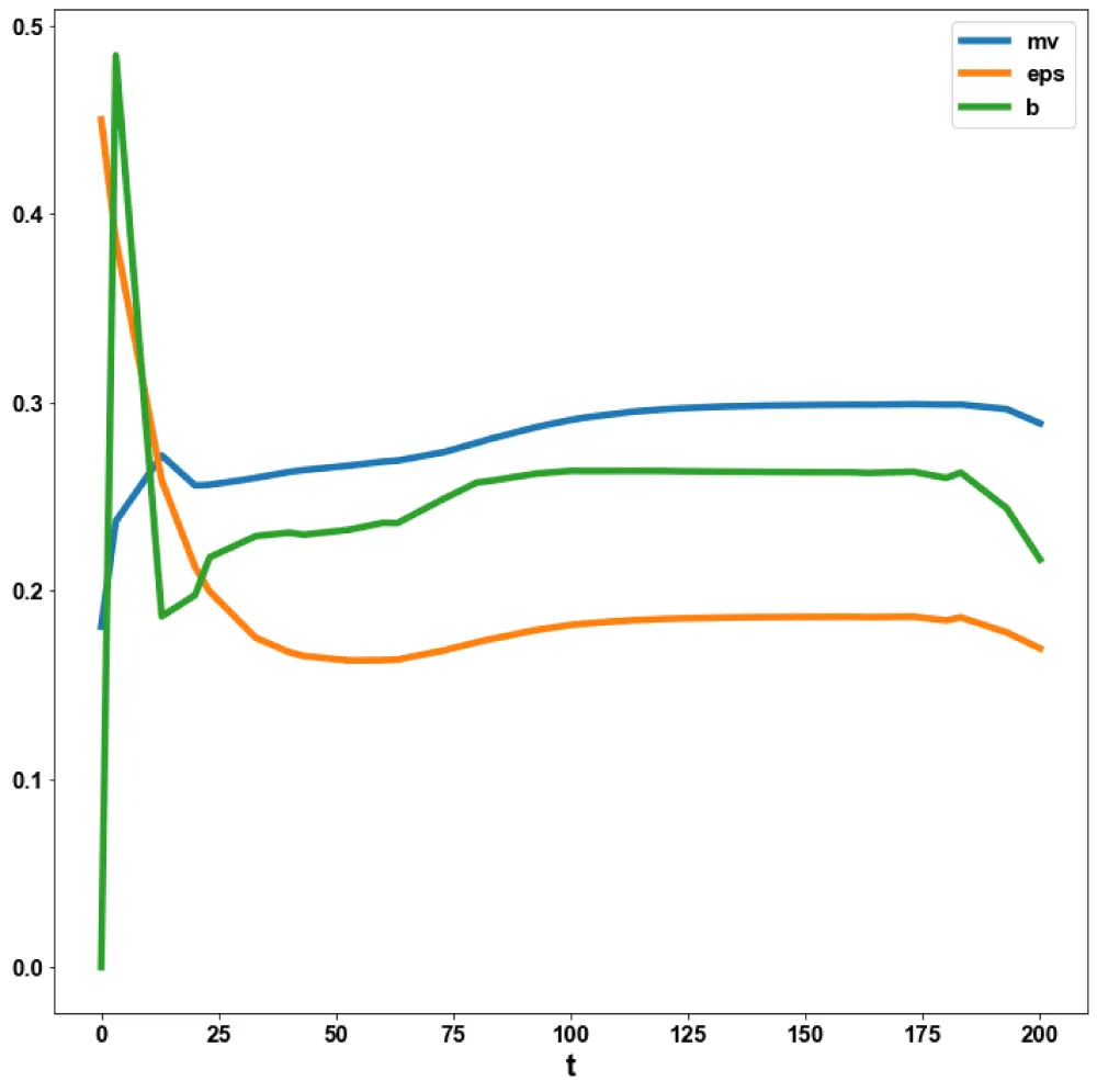
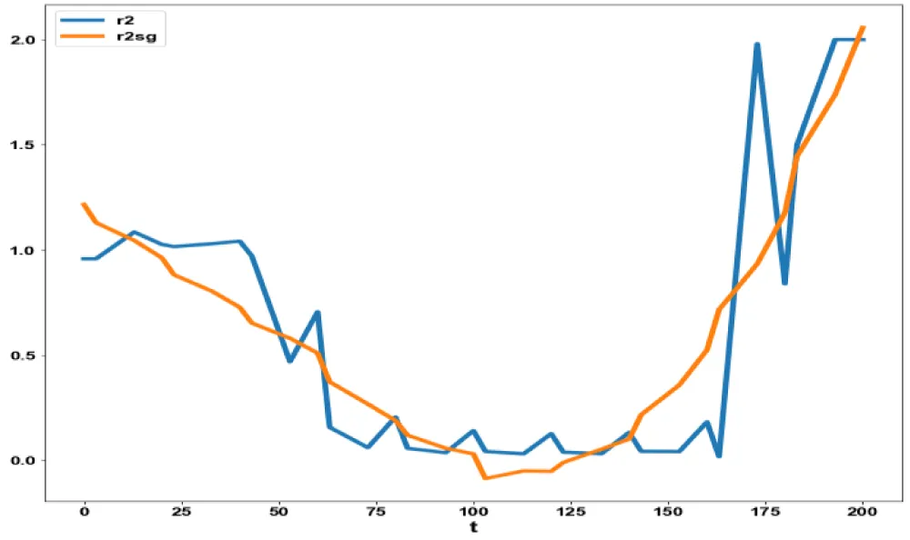
(bl,bpbl,eps,b,bpb,mv,r₂) Values of (13.2359, 0, 0.1860, 0.2626, 0.1287, 0.2987, 0.1976). This is shown in Figure 1. The MNLMPC calculations were minimized individually and led to values of 20.5914 and 0.21552. r₂ was the control parameter. The multiobjective optimal control problem will involve the minimization of the subject to the equations governing Model 1. This led to a value of zero (the Utopia solution). The MNLMPC control value (r₂) was 00.95777. Figures 2,3 show the various MNLMPC profiles. Figure 4 shows the control profile of r2. This profile exhibited noise, which was remedied by using the Savitzky-Golay filter to produce the smooth version of r₂ (r₂sg).

Figure 1: Bifurcation analysis Probiotic model 1 (indicating branch point).

Figure 2: MNLMPC Probiotic model 1 (bl, bpbl,bpb).

Figure 3: MNLMPC Probiotic model 1 (mv, eps,b).

Figure 4: MNLMPC Probiotic model 1 (r2, r2sg)(r2sg is the smooth version of r2 obtained by using the Savitzky Golay Filter).

Probiotic model 2

When r1 was used as the bifurcation parameter, a branch point was located at

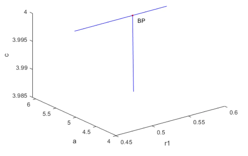
(b1,b2,c,a,r1) values of (0; 0; 4.000000 5.084746; 0.532881). This is shown in Figure 5.

Figure 5: Bifurcation analysis Probiotic model 2 (indicating branch point).

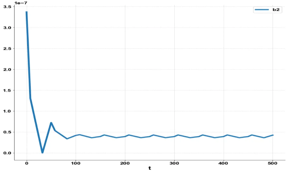
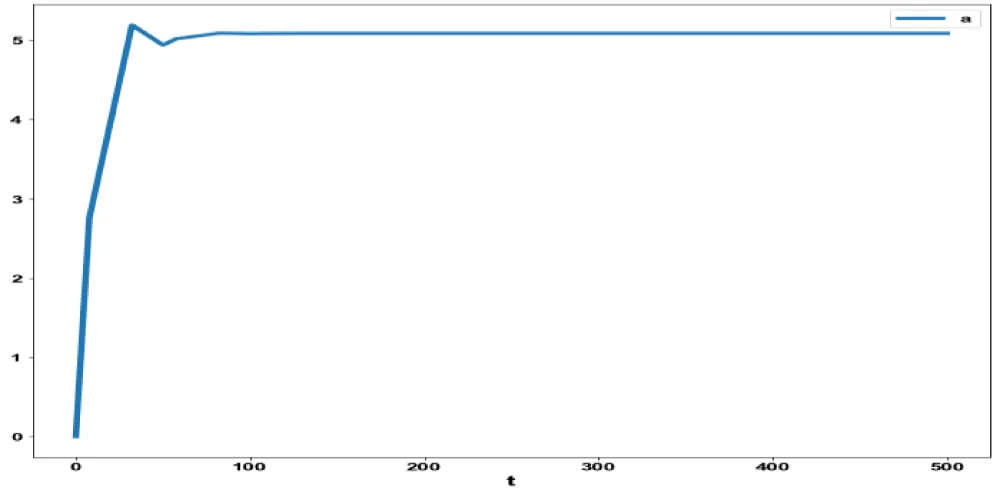
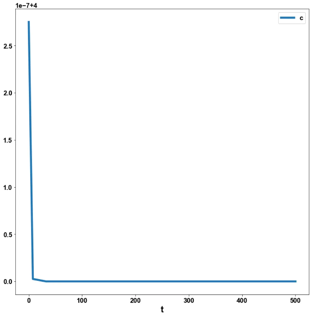
For the MNLMPC calculations, ${\displaystyle \sum _{t_{i=0}}^{t_i=t_f}b2(t_i)},{\displaystyle \sum _{t_{i=0}}^{t_i=t_f}c(t_i)},{\displaystyle \sum _{t_{i=0}}^{t_i=t_f}a(t_i)}$ were minimized individually and led to values of 0, 8, and 5.0847. R1 was the control parameter. The multiobjective optimal control problem will involve the minimization of the subject to the equations governing Model 1. This led to a value of zero (the Utopia solution). The MNLMPC control value (1) was 0.2185649. Figures 6-9 and 3 show the various MNLMPC profiles.

Figure 6: MNLMPC Probiotic model 1(b2).

Figure 7: MNLMPC Probiotic model 1(a).

Figure 8: MNLMPC Probiotic model 1(c).

Discussion of results

Theorem

If one of the functions in a dynamic system is separable into two distinct separable functions, a branch point singularity will occur in the system.

Proof

Consider a system of equations.

$\frac{dx}{dt}=f(x,\alpha )\text{ (14)}$

α Is the bifurcation parameter. Define the matrix A as

$A=[\frac{\partial f}{\partial y}]\text{ (15)}$

The tangent at any point y; ( $z=[z_1,z_2,z_3,z_4,\mathrm{....}{z}_{n+1}]$ ) must satisfy

$Az=0\text{ (16)}$

For a branch bifurcation point (Branch point from now on) (BP), the matrix must be singular. Let any of the functions (in the set f(y)), f_i, be separable into 2 functions φ₁, φ₂ as

$f_i={\varphi }_1{\varphi }_2\text{ (17)}$

At steady-state $f_i(y)=0$ and this will imply that either or both must be 0. This implies that the two branches will meet at a point where both are 0.

At this point, the corresponding row in the matrix B would be

$[\frac{\partial f_i}{\partial y_k}]\text{ (18)}$

However,

$[\frac{\partial f_i}{\partial y_k}={\varphi }_1(=0)\frac{\partial {\varphi }_2}{\partial y_k}+{\varphi }_2(=0)\frac{\partial {\varphi }_1}{\partial y_k}=0(\forall k=1.,,n)\text{ (19)}$

This implies that every element in the row would be 0, and hence the matrix B would be singular. The singularity in B implies that there exists a branch point.

In the probiotic model 1, a branch point was located at

(bl,bpbl,eps,b,bpb,mv,r₂) values of (13.2359, 0, 0.1860, 0.2626, 0.1287, 0.2987, 0.1976)

(Here, the two distinct functions can be obtained from the second ODE in probiotic model 1

$\frac{d(bpbl)}{dt}=r_2(bpbl)\left(1-\frac{\left(bpbl+\left({\alpha }_2*bl\right)\right)}{k2}\right)-eps(k)bpbl\text{ (20)}$

The two distinct functions are

$bpbl=0\text{ (21)}$

and

$r_2\left(1-\frac{\left(bpbl+\left({\alpha }_2*bl\right)\right)}{k2}\right)-eps(k)\text{ (22)}$

The values satisfy both the equations and computationally validate the theorem.

In the probiotic model 2, a branch point was located at the values (b1, b2, c, a, r1) of (0, 0, 4.000000, 5.084746, 0.532881).

(Here, the two distinct functions can be obtained from the first ODE in probiotic model 2,

$\frac{d(b_1)}{dt}=(1-\left(\frac{b_1+\left({\alpha }_1{b}_2\right)}{k}\right)r_1(b_1)+\left({\beta }_0{b}_1\right)-\left(\left({\beta }_1+{\gamma }_1\right)(a)b_1\right)-\left({\mu }_1{b}_1\right)\text{ (23)}$

The two distinct functions are

$b_1=0\text{ (24)}$

and

$(1-\left(\frac{b_1+\left({\alpha }_1{b}_2\right)}{k}\right)r_1+\left({\beta }_0\right)-\left(\left({\beta }_1+{\gamma }_1\right)(a)\right)-\left({\mu }_1\right)=0\text{ (25)}$

Setting

$\begin{array}{l}k=40;{\alpha }_1=0.1;{\beta }_0=0.14;{\beta }_1=0.016;{\mu }_1=0.5;{\gamma }_1=0.018;b_1=0,b_2=0,c=4,\\ a=5.084746,r_1=0.532881\end{array}$

Satisfies both the equations and validates the theorem.

Additionally, the MNLMPC calculations in both models converge to the Utopia solution, justifying the analysis of Sridhar [29].

Conclusion

Bifurcation analysis and multiobjective nonlinear control (MNLMPC) studies in two probiotic therapy models. The bifurcation analysis revealed the existence and branch points in both models. The branch points (which cause multiple steady-state solutions from a singular point) are very beneficial because they enable the Multiobjective nonlinear model predictive control calculations to converge to the Utopia point (the best possible solution) in the models. It is proven (with computational validation) that the branch points were caused because of the existence of two distinct separable functions in one of the equations in each dynamic model. A theorem was developed to demonstrate this fact for any dynamic model. A combination of bifurcation analysis and Multiobjective Nonlinear Model Predictive Control (MNLMPC) for dynamic models involving probiotic therapy is the main contribution of this paper.

Data availability statement

All data used is presented in the paper

Conflict of interest

The author, Dr. Lakshmi N Sridhar, has no conflict of interest.

Dr. Sridhar thanks Dr. Carlos Ramirez and Dr. Suleiman for encouraging him to write single-author papers.

1. Mattar AF, Drongowski RA, Coran AG, Harmon CM. Effect of probiotics on enterocyte bacterial translocation in vitro. Pediatr Surg Int. 2001;17:265–8. Available from: https://doi.org/10.1007/s003830100591
2. Dani C, Biadaioli R, Bertini G, Martelli E, Rubaltelli FF. Probiotics feeding in prevention of urinary tract infection, bacterial sepsis and necrotizing enterocolitis in preterm infants: a prospective double-blind study. Biol Neonate. 2002;82(2):103–8. Available from: https://doi.org/10.1159/000063096
3. Millar M, Wilks M, Costeloe K. Probiotics for preterm infants? Arch Dis Child Fetal Neonatal Ed. 2003;88:F354–8. Available from: https://doi.org/10.1136/fn.88.5.f354
4. Bin-Nun A, Bromiker R, Wilschanski M, Kaplan M, Hammerman C, et al. Oral probiotics prevent necrotizing enterocolitis in very low birth weight neonates. J Pediatr. 2005;147(2):192–6. Available from: https://doi.org/10.1016/j.jpeds.2005.03.054
5. Land MH, Rouster-Stevens K, Woods CR, Cannon ML, Cnota J, et al. Lactobacillus sepsis associated with probiotic therapy. Pediatrics. 2005;115(1):178–81. Available from: https://doi.org/10.1542/peds.2004-2137
6. Szajewska H, Setty M, Mrukowicz J, Guandalini S. Probiotics in gastrointestinal diseases in children: hard and not-so-hard evidence of efficacy. J Pediatr Gastroenterol Nutr. 2006;42(5):454–75. Available from: https://doi.org/10.1097/01.mpg.0000221913.88511.72
7. Hammerman C, Kaplan M. Probiotics and neonatal intestinal infection. Curr Opin Infect Dis. 2006;19(3):277–82. Available from: https://doi.org/10.1097/01.qco.0000224823.73223.29
8. Barclay AR, Stenson B, Simpson JH, Weaver LT, Wilson DC. Probiotics for necrotizing enterocolitis: a systematic review. J Pediatr Gastroenterol Nutr. 2007;45:569–76. Available from: https://doi.org/10.1097/mpg.0b013e3181344694
9. AlFaleh K, Bassler D. Probiotics for prevention of necrotizing enterocolitis in preterm infants. Cochrane Database Syst Rev. 2008;(1):CD005496. Available from: https://doi.org/10.1002/14651858.cd005496.pub4
10. Lin H, Hsu C, Chen H, Chung M, Hsu J, Lien R, et al. Oral probiotics prevent necrotizing enterocolitis in very low birth weight preterm infants: a multicenter, randomized controlled trial. Pediatrics. 2008;122(4):693–700. Available from: https://doi.org/10.1542/peds.2007-3007
11. Claud EC, Walker WA. Bacterial colonization, probiotics, and necrotizing enterocolitis. J Clin Gastroenterol. 2008;42 Suppl 3 Pt 1:S46–52. Available from: https://doi.org/10.1097/mcg.0b013e31815a57a8
12. Arciero JC, Ermentrout GB, Upperman JS, Vodovotz Y, Rubin JE. Using a mathematical model to analyze the role of probiotics and inflammation in necrotizing enterocolitis. PLoS One. 2010;5(4):e10066. Available from: https://doi.org/10.1371/journal.pone.0010066
13. Zhang YJ, Li S, Gan RY, Zhou T, Xu DP, Li HB. Impacts of gut bacteria on human health and diseases. Int J Mol Sci. 2015;16(4):7493–519. Available from: https://doi.org/10.3390/ijms16047493
14. Ahmed M, Jawad S. Bifurcation analysis of the role of good and bad bacteria in the decomposing toxins in the intestine with the impact of antibiotic and probiotics supplements. In: Fifth International Conference on Applied Sciences: ICAS2023. Available from: https://doi.org/10.1063/5.0209388
15. Dhooge A, Govaerts W, Kuznetsov AY. MATCONT: A MATLAB package for numerical bifurcation analysis of ODEs. ACM Trans Math Softw. 2003;29(2):141–64. Available from: https://dl.acm.org/doi/10.1145/779359.779362
16. Dhooge A, Govaerts W, Kuznetsov YA, Mestrom W, Riet AM. CL_MATCONT: A continuation toolbox in MATLAB. 2004.
17. Kuznetsov YA. Elements of applied bifurcation theory. New York: Springer; 1998. Available from: https://www.ma.imperial.ac.uk/~dturaev/kuznetsov.pdf
18. Kuznetsov YA. Five lectures on numerical bifurcation analysis. Utrecht University; 2009.
19. Govaerts WJF. Numerical methods for bifurcations of dynamical equilibria. Philadelphia: SIAM; 2000. Available from: https://epubs.siam.org/doi/pdf/10.1137/1.9780898719543.fm
20. Dubey SR, Singh SK, Chaudhuri BB. Activation functions in deep learning: A comprehensive survey and benchmark. Neurocomputing. 2022;503:92–108. Available from: https://doi.org/10.1016/j.neucom.2022.06.111
21. Kamalov AF, Nazir M, Safaraliev AK, Cherukuri R, Zgheib R. Comparative analysis of activation functions in neural networks. In: 2021 28th IEEE International Conference on Electronics, Circuits, and Systems (ICECS). Dubai, United Arab Emirates. 2021;1–6. Available from: https://ieeexplore.ieee.org/document/9665646
22. Szandała T. Review and comparison of commonly used activation functions for deep neural networks. ArXiv. 2020. Available from: https://link.springer.com/chapter/10.1007/978-981-15-5495-7_11
23. Sridhar LN. Bifurcation analysis and optimal control of the tumor macrophage interactions. Biomed J Sci Tech Res. 2023;53(5). Available from: https://biomedres.us/pdfs/BJSTR.MS.ID.008470.pdf
24. Sridhar LN. Elimination of oscillation causing Hopf bifurcations in engineering problems. J Appl Math. 2024;2(4):1826. Available from: https://doi.org/10.59400/jam1826
25. Flores-Tlacuahuac A, Morales P, Riveral Toledo M. Multiobjective nonlinear model predictive control of a class of chemical reactors. Ind Eng Chem Res. 2012;51(16):5891–9. Available from: https://pubs.acs.org/doi/abs/10.1021/ie201742e
26. Hart WE, Laird CD, Watson JP, Woodruff DL, Hackebeil GA, Nicholson BL, et al. Pyomo: Optimization modeling in Python. 2nd ed. Vol. 67. Available from: https://link.springer.com/book/10.1007/978-3-030-68928-5
27. Wächter A, Biegler L. On the implementation of an interior-point filter line-search algorithm for large-scale nonlinear programming. Math Program. 2006;106:25–57. Available from: https://doi.org/10.1007/s10107-004-0559-y
28. Tawarmalani M, Sahinidis NV. A polyhedral branch-and-cut approach to global optimization. Math Program. 2005;103(2):225–49. Available from: https://citeseerx.ist.psu.edu/document?repid=rep1&type=pdf&doi=07d4f1c68c9952a41147f7125fc968614f451707
29. Sridhar LN. Coupling bifurcation analysis and multiobjective nonlinear model predictive control. Austin Chem Eng. 2024;10(3):1107. Available from: https://austinpublishinggroup.com/chemical-engineering/fulltext/ace-v11-id1107.pdf
30. Upreti SR. Optimal control for chemical engineers. Boca Raton: Taylor and Francis; 2013. Available from: https://doi.org/10.1201/b13045