Damage model of turbine rotor based on DPLS

In today’s society, the development of electric power industry is one of the important conditions for the economic construction of a country. Therefore, it is of great theoretical significance and value to carry out the research on the damage assessment of turbine rotor. The damage of the turbine rotor is directly related to the process quality, material performance, operation conditions of the equipment itself, and also closely related to the performance of the controller. According to the existing data and starting conditions, a dynamic partial least square prediction model is established and analyzed in this paper, so as to effectively evaluate the stress and damage of the turbine rotor. Before the establishment of dynamic partial least squares model, people study the change law of stress value and damage value mainly through complex mathematical formulas and inconvenient finite element analysis software. After the establishment of dynamic partial least squares model, the staff only need to input the input data (speed, temperature, back pressure) to the model to get the stress. The function is also realized in this paper.

Introduction

Research background and research status

The working environment of the steam turbine rotor is very bad, the thermal stress changes greatly, plus its own moment of inertia is large, there are many stress concentra­tion parts, its material performance, geometry and operation conditions have a great impact on the normal operation of the steam turbine [1]. Rotor is the most dangerous part in the whole unit, its life determines the life of the whole turbine unit. Because when the rotor is rotating at high speed, with the change of unit load, the rotor itself will produce large al­ternating thermal stress. Therefore, the life of the whole unit can be controlled by controlling the thermal stress change of the rotor.

At present, the research focus in the field of steam tur­bine life assessment and management mainly focuses on the calculation method of life loss and the research of various nonlinear damage accumulation methods in the process of start-up and shut-down [2].

During the start-up and operation of steam turbine, the thermal stress and mechanical stress on the rotor gradually change, involving many process variables, including steam pressure, steam temperature, steam temperature change rate, rotor speed, etc., which belongs to the transient condition of steam turbine [3]. The variation of these variable parameters has a direct impact on the service life of turbine rotor metal materials. For example, the large change of steam temper­ature will cause great thermal stress and metal fatigue dam­age, while the continuous high temperature and high pres­sure will cause the creep damage of rotor metal materials [4].

During the transient condition, the heat transfer process inside the steam turbine components is unstable, which leads to the uneven temperature distribution inside the metal, thus causing the thermal stress inside the metal. In order to con­trol the life consumption of steam turbine components, it is necessary to control the thermal stress, that is, to control the change speed of steam turbine parameters under transien­t conditions [5].

At present, there are two kinds of life analysis and pre­diction methods for steam turbine at home and abroad, one is one-dimensional analysis method, the other is numeri­cal analysis method [6]. The rotor body is simplified as an infinite cylinder by one-dimensional analytical method [7]. The temperature change of each part is calculated by one-dimensional unsteady heat conduction differential equation, and then the thermal stress is calculated by volume average temperature difference [8]. This method takes into account the radial temperature difference of the rotor, the calculation process is simple and practical, and it can be used for online monitoring of turbine rotor damage. However, the method simplifies the rotor as a cylinder, which not only ignores the influence of the geometry on the stress concentration, but also directly treats the heat transfer conditions on the rotor surface and the physical characteristics of the metal as con­stants, which affects the calculation accuracy. With the rapid development of computer technology, the numerical analy­sis technology represented by the finite element analysis has been highly valued and widely used in the subject of Turbine Damage Assessment and life prediction [9].

For steam turbine in thermal power plant, the ultimate goal of optimization is to reduce the stress value and start-up time of rotor. In the unit, the rotor of steam turbine is an important part, which carries the energy and torque [10]. The safety of steam turbine unit is mainly determined by the quality of turbine rotor. Reducing the start-up time of the equipment is a decisive factor while ensuring that the stress value of the turbine rotor is less than the yield limit value of the rotor material. From a few years ago to now, the quality of life has improved significantly, the grid capacity has increased significantly, so the peak value of the grid has been increasing [11]. Frequent peak shaving operation means frequent start-up and shutdown of the steam turbine unit. The change of working condition of steam turbine unit will cause the damage of rotor material, thus shortening the life of the unit [12]. The parameters of steam turbine will change greatly during start-up. Among them, the change of temperature parameter is the most important [13]. It will make the rotor produce a force, which is called thermal stress. At the same time, it will make the metal material deform, mainly in the form of expansion deformation [14]. Once the thermal stress exceeds the yield limit of the rotor material, the high-temperature components, mainly the turbine rotor, will produce certain damage, which will eventually bring some security risks [15].

The needs of today’s society should be met, so it is necessary and very important to study the rapid start-up process. The start and stop of steam turbine depends on how long it can be used, which means that it directly affects the life of the unit. After a detailed study of the start and stop of the steam turbine unit, a curve of start-up is given and used to guide the unit, which can improves security and economy at the same time. In brief, the start-up optimization of steam turbine is to optimize a function. At the same time, this function has constraint conditions. Generally speaking, the start-up time is the shortest and the stress is within a reasonable range\cite{C04}.

Before that, there were many ways to optimize start-up of unit. It is impractical to measure and test the input data in the actual power plant, so using complex simulation software is the most commonly used method to evaluate the solution.For an axisymmetric body, such as a steam turbine rotor, whose geometry is irregular and boundary conditions vary greatly, it is necessary to apply numerical method to obtain accurate calculation results [16]. The rotor is considered as an ax­isymmetric two-dimensional computational model, and the complex geometric continuum is discretized. The heat re­lease coefficient and material properties of the medium on the surface of the rotor are treated as variables with starting time. The Finite Element Method (FEM) is the most com­monly used numerical method for thermal stress calculation. It is developed on the basis of energy method and differ­ence method, and has both advantages. The essence of the finite element method is to use the variational calculation in the element and the overall synthesis to replace the differ­ential equation solution [17]. As long as the partition element is small enough, the result can be obtained with enough accura­cy by using simple linear interpolation function. Moreover, the mesh division is flexible and the adaptability to irregular boundary is good.

Research objective

The prediction process of dynamic partial least squares is dynamic, which can change with the input data, and directly reflect the stress and damage data of turbine rotor in the whole start-up process. In the past, only three-dimensional modeling of turbine rotor was carried out in the research of steam turbine, which was imported into the finite element analysis software (commercial ANSYS, ADINA, etc.) through the finite element analysis The software calculates the thermal stress, and then calculates the effective stress through the fourth strength criterion formula (the effective stress refers to the coupling superposition of thermal stress and centrifugal stress). Finally, the damage value is calculated through the damage calculation formula. The whole process is very troublesome and complex, there will be a lot of work and time-consuming, and it can be well avoided by using the partial dynamic least squares model These problems only need to input the start-up data of the turbine rotor, and can be analyzed through the model.

Structure of turbine starting system

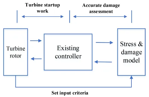
At present, in order to analyze the actual working condition more effectively and economically, the system structure model which is basically consistent with the actual working condition has been established in most industrial occasions. Through the analysis and experiment of the structure model, the working state and efficiency of the system can be judged. However, the accuracy and efficiency of different structural models are different. In this paper, a high precision stress damage model of steam turbine starting system is established. Figure 1 shows the structure diagram of the interaction between the stress damage model and existing controllers and plants. Based on the actual starting conditions, the model can accurately estimate the stress value and the damage value of the steam turbine during the start-up and cold state. So that it can accurately evaluate the start-up damage without affecting the working conditions of the unit.

Figure 1: Schematic diagram of system structure model.

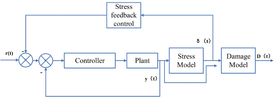
Combined with the above, this paper proposes the scheme as shown in Figure 2, the small feedback loop in the figure is the control system designed for the dynamic performance of the whole system under the existing actual working conditions. The stress model, damage model and stress feedback control are the new modules introduced in this paper.

Figure 2: Model control structure details.

r(t) is the input of system operation, y(t) is the input of plant rotor working condition, δ(t) is stress output, D(t) is damage output. It should be noted that the controller does not need to be changed. The stress feedback control is introduced into the structural model to judge the load level of the unit according to the monitoring of the corresponding stress value, so as to extend the service life of the unit. The damage model is used to evaluate the damage value in the process of unit startup. This structural model is suitable for online implementation, and its features include:

1. Stress model and damage model belong to the level of accurate life assessment, which can give more accurate assessment of stress value and damage value.

2. The evaluation is faster and more efficient.

3. The system can adjust the input and output according to the feedback of stress value and damage value, so as to prolong the life of the unit.

Establishment of online damage assessment model based on DPLS

The working environment of the steam turbine rotor is very bad, the thermal stress changes greatly, plus its own moment of inertia is large, there are many stress concentra­tion parts, its material performance, geometry and operation conditions have a great impact on the normal operation of the steam turbine. Rotor is the most dangerous part in the whole unit, its life determines the life of the whole turbine unit. Because when the rotor is rotating at high speed, with the change of unit load, the rotor itself will produce large al­ternating thermal stress. Therefore, the life of the whole unit can be controlled by controlling the thermal stress change of the rotor.

The rotor of the steam turbine is the worst part of the working environment in the whole working process of the steam turbine unit. During the whole starting process of the unit, the thermal stress of the rotor changes the most, and there are many stress concentration parts of the rotor. In addition, the material performance, starting conditions and other conditions have a great impact on the normal operation of the steam turbine. Among the components of the whole unit, the most critical is the rotor of the turbine. The service life of the rotor basically determines the service life of the turbine unit. Therefore, the life of the whole turbine can be controlled by controlling the thermal stress of the turbine rotor. Up to now, most of the researches are on the calculation method of life loss and nonlinear damage accumulation method of steam turbine, but the accurate online control of steam turbine life is less.

At present, there are two methods to analyze and predict the life of steam turbine, one is analytical method, the other is numerical analysis method. One dimensional analytical method is to calculate the temperature change of each part through the differential equation of heat conduction, and then calculate the thermal stress through the volume average temperature difference. However, this method simplifies the rotor into a cylinder and ignores the concentrated effect of the geometric structure on the stress. The numerical analysis method represented by the finite element analysis is to establish a two or three-dimensional model, and then calculate and analyze its stress, so as to avoid over simplification and make the results more accurate.

Establishment and analysis of DPLS prediction model

The partial least squares method was first proposed by wold. It is a regression modeling method that multiple independent variables correspond to multiple dependent variables. Partial least square method decomposes independent variable x and dependent variable y of life loss, and extracts useful data from them.

In the start-up process of steam turbine, the high temperature and high pressure steam drives the turbine rotor to rotate, steam and temperature are continuously changing, and there is a high correlation between parameters. In order to maximize the use of finite element analysis data and more truly reflect the impact of process variables on the life of turbine rotor, this paper adopts DPLS regression modeling method, that is, in the input and output The data of dependent and independent variables are included in the matrix, and the expanded matrix is regressed by partial least squares.

Define input variables, output variables and matrices $u_t$ ,$y_t$ and $x_t^T$ .

$u_t={\left[\begin{array}{ccc}{P}_t& T_t& N_t\end{array}\right]}^T(1)$

$x_t{}^T=\left[\begin{array}{ccc}{u}_t& u_t{}^2& y_t{}^2\end{array}\right](3)$

In this way, the input matrix X can be constructed as:

$X={\left[\begin{array}{cccc}{x}_t{}^T& x_{t-1}{}^T& \cdots & x_{t-n}{}^T\\ x_{t-1}{}^T& x_{t-2}{}^T& \cdots & x_{t-n-1}{}^T\\ ⋮& ⋮& \ddots & ⋮\\ x_{t-m}{}^T& x_{t-1-m}{}^T& \cdots & x_{t-n-m}{}^T\end{array}\right]}^T(4)$

At the same time, the output matrix Y can also be obtained:

$Y={\left[\begin{array}{cccc}{y}_t& y_{t-1}& \cdots & y_{t-n}\end{array}\right]}^T(5)$

In this paper, the design idea of partial least squares is to extract ti, i = 1,2..., from the independent variable X of turbine rotor. The $u_i$ is extracted from the dependent variable Y and the regression equation is established.

Firstly, the process variable matrix X and Y of the steam turbine rotor are processed. In this paper, the mean value and proportion are taken. The X matrix can be decomposed into the product of the score vector H and the load vector I, plus the form of the residual matrix F, the Y matrix can be decomposed into the product of the score vector K and the load vector R, plus the form of the residual matrix E:

$X={\displaystyle \sum _{j=1}^a{t}_j}{p}_j{}^T+F_{a+1}=H{I}^T+F_{a+1}(6)$

$Y={\displaystyle \sum _{j=1}^a{u}_j}{q}_j{}^T+E_{a+1}=K{R}^T+E_{a+1}(7)$

where H,$\subseteq$ $R^{n*a}$ I $\subseteq$ $R^{m*a}$ , K$\subseteq$ $R^{N*a}$ , R$\subseteq$ $R^{\text{p}*a}$ , F$\subseteq$ $R^{\text{n}*\text{m}}$ , E$\subseteq$ $R^{\text{n}*\text{p}}$ , a is the number of main elements. $t_j,p_j,u_j,q_j$ is the partition vector of the j-th column of matrix H, I, K, R.

If $\alpha =min(m,n)$ then F and E are 0, in this way, PLS will be reduced to the ordinary least square method. If $\alpha \le min(m,n)$ then through the process of principal component analysis, the goal of reducing dimension and collinearity can be achieved.

By regression analysis of the score vectors ${\tilde{\text{u}}}_j$ and P of Y and X matrices, including:

${\tilde{\text{u}}}_j=L_j(q^{-1})t_j(8)$

where $L_j(q^{-1})t_j$ is the dynamic regression coefficient, j=1,2,...,a. The form of matrix can be expressed as:

${\tilde{U}}_j=HL(q^{-}1)(9)$

$L(q^{-1})=\left[\begin{array}{ccccc}{L}_1(q^{-1})& 0& 0& \cdots & 0\\ 0& L_2(q^{-1})& 0& \cdots & 0\\ ⋮& 0& ⋮& \ddots & 0\\ 0& 0& 0& \cdots & L_a(q^{-1})\end{array}\right](10)$

If ${\tilde{U}}_j$ is introduced into ${\tilde{U}}_j$ , the residual matrix will be changed, as follows:

$Y=HL(q^{-1})R^T+\overline{E}(11)$

Where $\stackrel{-}{E}$ is the prediction error matrix, The criterion for selecting matrix $L_j(q^{-1})$ is to minimize the two norm of matrix $\stackrel{-}{E}$ . The form of score vector matrix of input-output matrix is defined as$K={\left[\begin{array}{cccc}{k}_1{}^T,& k_2{}^T,& \cdots & k_n{}^T\end{array}\right]}^T,U={\left[\begin{array}{cccc}{u}_1{}^T,& u_2{}^T,& \cdots & u_n{}^T\end{array}\right]}^T.$

The input and output measurements are:

$x_t=It+f_{t(a+1)}(12)$

$y_t=Ru+e_{t(a+1)}(13)$

$t=I_2{x}_t-I_2{f}_{t(a+1)}(14)$

t is the loading matrix after adding the new test input value. Bring in the formula to get:

$y_t=RL(q^{-1})t+e_{t(a+1)}(15)$

$y_t=RL(q^{-1})I_2{x}_t-RL(q^{-1})I_2{f}_{t(a+1)}+e_{t(a+1)}(16)$

Determine the following conditions:

$\left\{\begin{array}{c}{a}_t={(f_{t(a+1)}^T,e_{t(a+1)}^T)}^T\\ A(q^{-1})=RL(q^{-1})I_2\\ B(q^{-1})=[-RL(q^{-1})I_{2}T]\end{array}\right\}(17)$

get:

$y_t=A(q^{-1})x_t+B(q^{-1})a_t(18)$

The input variables are steam temperature, steam pressure, rotor speed, and the output is turbine rotor adjustment low cycle fatigue life damage of the root of the segment. It can be seen from the above analysis that the factors affecting the low cycle fatigue life of the turbine rotor are the current steam temperature value, the past temperature value (used to calculate the temperature change rate), the current steam pressure, the past steam pressure, the current speed value, the past speed value, the square of the speed value, the square of the past speed, the product of the pressure and speed, and the past value of the product of the pressure and speed.

Establishment of damage model

In this section, taking the impulse starting process of 300MW turbine as an example, the second power of dynamic deviation is analyzed. In the process of life prediction of steam turbine rotor, the mathematical model for life evaluation of control system is obtained, and the life loss data is predicted. In dynamic PLS model, both input and output variables are required to be measurable. However, the low cycle fatigue damage of turbine rotor is not measurable. Therefore, it is necessary to build an online calculation model of observed parts under specific working conditions to obtain damage data.

The low cycle fatigue damage of steam turbine can be decomposed into a dynamic linear model and a static nonlinear model. The key point is to identify the dynamic characteristics of temperature and stress. In the real-time monitoring of damage, these information are the basis of making decisions and controlling actions. Because of the complex physical mechanism of metal low cycle fatigue damage, it is very difficult to write its mathematical model directly. In this section, the rotor metal damage model of 300MW steam turbine during impulse running is established by nonlinear decomposition and model identification based on finite element simulation data.

In order to establish the on-line monitoring model of rotor metal, it is necessary to identify the transfer function of main steam temperature to rotor surface temperature G1 and the transfer function of heat flow density to thermal stress G₂. These two transfer functions can be inferred from the temperature data of the finite element analysis software:

The temperature data used in this paper is the data optimized by genetic algorithm according to the results under the starting curve of the original working condition. First, calculate the temperature and temperature output curve under the original working condition curve, and calculate G₁₁ and G₂₂.

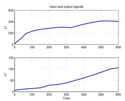
The following is the fitting process of the transfer function. Through the system identification toolbox of MATLAB, the transfer function shown in formula 19 and formula 20 can be obtained. The accuracy of the transfer function is 98.23% Figure 3.

Figure 3: System identification results.

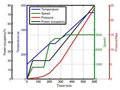
The starting curve of the original working condition is shown in the Figure 4 below:

Figure 4: Temperature data curve.

After fitting the data, G₁₁ and G₂₂ are as follows:

$G_{11}(s)=\frac{0.1224s-0.07515}{s^2-0.3934s-0.5587}(19)$

$G_{22}(s)=\frac{1198s-1196}{s^3-1.011s^2-0.7584s+0.77}(20)$

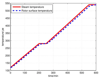
In this paper, the optimized results are used. The optimized temperature curve and temperature output curve are shown in the Figure 5 below:

Figure 5: Optimized temperature data curve.

The resulting transfer function is:

$G_1(s)=\frac{0.122741s-0.07881}{s^2-0.3854s-0.5782}(21)$

$G_2(s)=\frac{1284s-1249}{s^3-1.214s^2-0.7876s+0.82}(22)$

The optimized results greatly shorten the start-up time of the steam turbine unit. However, through comparison, the parameters of the transfer function have some changes, but the data changes little.

In this paper, according to the consideration of different working conditions, the temperature rise rate of the cold start-up curve under the real working condition is changed by using the finite element analysis software, and the corresponding thermal stress value is obtained. Then, the obtained thermal stress value is derived. Combined with the above two formulas, it is compared with the off-line calculation results to verify the feasibility of the model.

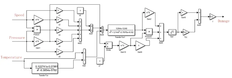
In this way, the stress of the turbine rotor can be modeled as damage. The stress and damage model is shown in the Figure 6 below:

Figure 6: Stress and damage models.

After the start of the impulse process, a large number of high temperature and high pressure steam enter the cylinder, and heat is continuously released on the rotor surface, resulting in the increasing thermal stress of the rotor, so the real-time data of low cycle fatigue damage is maintained in a high level data fluctuation.

Model simulation results and analysis

The input variables are steam temperature, steam pressure, rotor speed, and the output is turbine rotor adjustment Low cycle fatigue life damage of the root of the segment. It can be seen from the above analysis that the factors affecting the low cycle fatigue life of the turbine rotor are the current steam temperature value, the past temperature value (used to calculate the temperature change rate), the current steam pressure, the past steam pressure, the current speed value, the past speed value, the square of the speed value, the square of the past speed, the product of the pressure and speed, and the past value of the product of the pressure and speed.

Model simulation results

In the process of starting, stopping and changing working conditions of steam turbine, the rotor of steam turbine must bear huge temperature changes, which will cause uneven heating of rotor metal and generate thermal stress. During the start-up process of steam turbine, the stress of rotor is the superposition of various forces, including thermal stress caused by temperature, centrifugal force caused by rotation of rotor itself, pressure of working medium on rotor metal, bending moment caused by weight of rotor itself and torque caused by power transmission of steam turbine. Among them, the thermal stress value is the largest, which can reach the order of 100MPa, followed by centrifugal force, which can reach the order of 10MPa, and other force orders are very small. In order to ensure the calculation is simple, it can be ignored.

Therefore, thermal stress and centrifugal force are the main factors leading to plastic strain damage of rotor metal materials. Some experiments show that the damage of rotor metal in cold start is three times larger than that in warm start or warm start. The main difference between different operating conditions of steam turbine is temperature value, including initial temperature, end temperature and temperature change rate. These factors play an important role in damage accumulation.

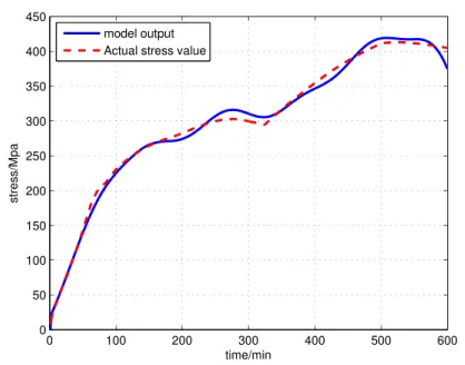
The input conditions under the actual working conditions are loaded into the design model, and the start-up curve includes the speed, load and time curves. The rotor stress data of the model is extracted and compared with the commercial ANSYS finite element analysis software. The comparison picture is shown in Figure 7. The model reflects the acceleration and load rate of each stage, and the corresponding damage value is obtained.

Figure 7: Comparison of actual stress and model output stress.

Under cold start-up conditions, large temperature gradients and thermal stresses often occur in key parts such as high pressure stage, regulating stage, intermediate pressure stage and steam seal. This is because, in these parts of the turbine rotor, the temperature change is very intense, and because of the specific geometry, these parts often appear stress concentration phenomenon. Therefore, in these parts, the combined stress often reaches a maximum value. The life loss of the turbine rotor depends on the loss accumulation of these key parts, so it is necessary to evaluate the rotor. In the case of life loss, it is only necessary to calculate the metal damage accumulation of these key parts.

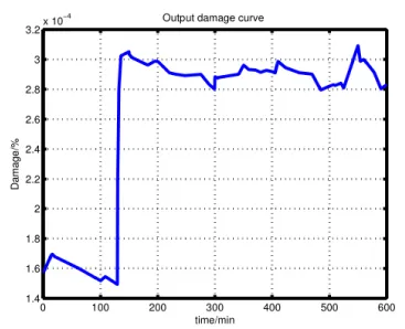
After starting the input conditions, the model calculates a set of damage values, and processes the damage data into the output picture as shown in the following Figure 8:

Figure 8: Output curve of damage value.

As can be seen in the figure, after the start of the impulse process, a large number of high temperature and high pressure steam enters the cylinder, and the heat is continuously released on the rotor surface, resulting in the increasing thermal stress of the rotor, so the real-time data of low cycle fatigue damage is maintained in a high level data fluctuation.

Analysis of model results

The results obtained from the model can be shown as follows: the results of the model are very close to the operation results of the actual plant, and the accuracy is a high level, through the analysis of the input and output data of the model, a relationship between the cold start-up curve and the thermal stress of the turbine rotor can be obtained. In the process of cold start-up, the thermal stress has a very direct relationship with the turbine rotor speed, steam temperature and steam pressure.

Conclusion

In view of the high spatial-temporal correlation of steam turbine system operation process data, a DPLS method is proposed in this chapter, which maximizes the covariance of steam parameter matrix and low cycle fatigue life loss, retains useful information, eliminates the correlation between variables, selects the same variables in different time series, reduces the dimension of simulation data from high-dimensional space, establishes an accurate model, and establishes a mathematical model Low cycle fatigue life loss model of steam turbine rotor. Finally, by comparing the experimental data with the simulation results, the online damage assessment model based on finite element technology is verified, and the effectiveness of DPLS algorithm in low cycle fatigue damage prediction of turbine rotor is verified. The inaccuracy of one-dimensional analysis method in the field is solved, while the inaccuracy of numerical analysis method in the field of life assessment is solved, which provides reference for the life prediction of turbine rotor It provides a new way of thinking in practice.

1. Zhang H, Xie D, Yu Y, Yu L (2016) Online optimal control schemes of inlet steam temperature during startup of steam turbines considering low cycle fatigue. Energy 117: 105-115. Link: https://bit.ly/3cRpOuS
2. Ji DM, Sun JQ, Dui Y (2017) The Optimization of the Start-up Scheduling for a 320 MW Steam Turbine. Energy 125: 345-355. Link: https://bit.ly/3dDmKl8
3. Nayebi A, Ranjbar H, Rokhgireh H (2013) Analysis of unified continuum damage mechanics model of gas turbine rotor steel: Life assessment. Proceedings of the Institution of Mechanical Engineers. Part L: Journal of Materials: Design and Applications 227: 216-225. Link: https://bit.ly/3fGUHE5
4. Zhang H, Xie D, Yu Y, Yu L (2016) Online optimal control schemes of inlet steam temperature during startup of steam turbines considering low cycle fatigue. Energy 117: 105-115. Link: https://bit.ly/3cRpOuS
5. Saboya Bautista I, Egido I, Lobato Miguelez E (2015) Performance Evaluation of Start-Up Decisions of Rapid-Start Units for AGC. IEEE T Power Syst 30: 1-9. Link: https://bit.ly/3rLGOah
6. Belkhir F, Cabo DK, Felgner F, Frey G (2015) Optimal Startup Control of a Steam Power Plant Using the JModelica Platform. IFAC-Papers OnLine 48: 204-209. Link: https://bit.ly/31NS6Ag
7. Zhang H, Xie D, Yu Y, Yu L (2016) Online optimal control schemes of inlet steam temperature during startup of steam turbines considering low cycle fatigue. Energy 117: 105-115. Link: https://bit.ly/3cRpOuS
8. He J, Chen J, Sun Q (2014) Effect of Loading Rate on Low-cycle Fatigue Properties of Turbine Rotor Steel. Procedia Materials Science 3: 1773-1779. Link: https://bit.ly/3sRtHWi
9. Nowak G, Rusin A (2016) Using the artificial neural network to control the steam turbine heating process. Appl Therm Eng 108: 204-210. Link: https://bit.ly/3dzYj8f
10. Poor H (1985) An Introduction to Signal Detection andEstimation. New York: Springer-Verlag, Chap. 4.
11. Kamiya A, Kawai K, Ono I, Kobayashi S (2002) Theoretical Proof of Edge Search Strategy Applied Power Plant Start-up Scheduling. IEEE T Syst, Man Cy. Part B: Cybernetics 32: 316-331. Link: https://bit.ly/3mjYwQU
12. Saboya Bautista I, Egido I, Lobato Miguelez E (2015) Performance Evaluation of Start-Up Decisions of Rapid-Start Units for AGC. IEEE T Power Syst 30: 1-9. Link: https://bit.ly/3miR1tq
13. Belkhir F, Cabo DK, Felgner F, Frey G (2015) Optimal Startup Control of a Steam Power Plant Using the JModelica Platform. IFAC-PapersOnLine 48: 204-209. Link: https://bit.ly/3rRNzqO
14. Zhang H, Xie D, Yu Y, Yu L (2016) Online optimal control schemes of inlet steam temperature during startup of steam turbines considering low cycle fatigue. Energy 117: 105-115. Link: https://bit.ly/3cRpOuS
15. Nowak G, Rusin A (2016) Using the artificial neural network to control the steam turbine heating process. Appl Therm Eng 108: 204-210. Link: https://bit.ly/3dzYj8f
16. Min JH, Lee Y (2005) Bankruptcy prediction using support vector machine with optimal choice of kernel function ACCEPTED MANUSCRIPT 19 parameters. Expert Syst Appl 28: 603-614. Link: https://bit.ly/3mnJ6vc
17. Jing J, Meng G, Sun Y (2003) An effective continuum damage mechanics model for creep-fatigue life assessment of a steam turbine rotor. Int J Pres Ves Pip 80: 389-396. Link: https://bit.ly/3cMgCrI