Alongshore sediment transport rate –measurement and comparison with empirical formulas and an Artificial Neural Network (ANN) model

The rate from alongshore sediment transport in the surf zone depends on the product of the local wave height and mean alongshore current speed. The aim of this article was to predict the alongshore sediment transport rate using a semi-empirical application of Artificial Neural Network (ANN) on the south coast of the Caspian Sea. This study reports the measurements of the alongshore sediment transport rate performed in the surf zone of the Noor coastal area located in the southern part of the Caspian Sea from September 2011 to June 2012. Further, alongshore sediment transport rates have been estimated by different famous semi-empirical formulas. On the other hand, an artificial neural network model was trained using three predominant parameters of sediment transport formulas including wave-breaking height (H_b), surf zone width (W), and alongshore current velocity (V). ANN models were able to show hidden laws of natural phenomena such as the sediment transport process. The results of ANN and some sediment transport rate formulas concerning alongshore sediment transport rate were compared with corresponding measured values. Sediment transport is still an evolving science because it depends on complex processes. It is worth mentioning that some of these processes have not been measured or fully understood. Therefore, it is necessary for engineers to pay attention to the fact that even the best forecasts available in the field of sediment transport have a wider margin of error than the forecasts expected in other disciplines and fields of science and engineering. The results show that the estimated value of alongshore sediment transport rate by Coastal Engineering Research Center (CERC), Walton and Bruno, Kamphuis formulas, and ANN model is 737.8 $\frac{m^3}{day}$ , 670.3 $\frac{m^3}{day}$ , 593.3 $\frac{m^3}{day}$ and 592.4 $\frac{m^3}{day}$ , respectively. Also, according to the results, the calculated R2 values, in the estimation of alongshore sediment transport rate for ANN model and CERC, Walton and Bruno, and Kamphuis formulas, are 0.99, 0.78, 0.75, and 0.66, while the Root Mean Squared Error (RMSE) values are 4.7 × 10^-4, 8.4 × 10^-3, 9.1 × 10^-2 and 2.4 × 10^-3, respectively.This work carried out in the framework of the SWOT 3MC research program, gives some insights into the complex behavior of tidal propagation in the Seine estuary and its non-stationary dynamics close to the river effects in response to extreme sea levels leading to coastal flooding.

Introduction

In recent decades, different empirical formulas have been presented to predict the coastal sediment transport rate by many researchers. Each of them has been calibrated and is used for a certain range of sediment grains, under limited conditions of bed sedimentation. An in-depth literature review revealed that one of the most used models for predicting the parallel shore sediment transport rate was based on Artificial Neural Network (ANN) techniques, due to its constantly high predictive ability compared to other approaches, i.e., linear models, which constitute one of the major’s motivation of our present investigation.

Prediction of coastal parallel sediment transport is an important objective of coastal engineers to determine erosion and sedimentation. Most scientists have struggled to find the experimental procedure to predict the rate of parallel shore sediment transport in the past decades; Although, because of the significant influence of random parameters and data, the existing experimental methods have offered completely different results and limited applications. The longshore sediment transport rate enters most coastal engineering designs. The longshore current generated by obliquely incident-breaking waves plays an important role in transporting sediment in the surf zone. The longshore current velocity varies across the surf zone, reaching a maximum value close to the wave-breaking point Galvin, 1967, Basco, 1982. For practical purposes, the average longshore current measured in the surf zone should be sufficient for estimating the longshore sediment transport rate (LSTR). LSTR is, in general, calculated using semi-empirical equations, which are mostly based on laboratory data (Shore Protection Manual, 1984). A sediment transport equation incorporating field data would, however, be more reliable for field application at a particular site. [1].

The formulas for the calculation of the parallel coast transport rate have been developed over several years. The Coastal Engineering Research Center (CERC) formula developed in 1973 by the U.S. Army Engineer Waterways Experiment Station (WES) and later updated in 1984 was based on the assumption that the rate of sediment transport is calculated only for the part induced by waves using the overall wave characteristics [2-4].

Sediment transport is still a science in evolution because it depends on complex processes. Some of these processes are not measured or fully understood; therefore. In fact, the prediction of precipitation transfer has been far more accurate compared to the prediction of other weather factors [5].

Wave breaking near coastal regions and currents are two main factors known for coastal sediment transport. Waves generate energy from the winds blowing on the surface of the water, and when they reach the break-point region they lose a large amount of energy. Wave breaking leads to disarray in the water column and movement of sediment [6].

The transport rate of sediment load which is carried by surface flow, is a main pattern in controlling river ecosystems and is one of the main parameters in the design, implementation, and utilization of hydraulic structures, irrigation, transfer and treatment of water, watershed management, and flood control. Given the importance of the sediment transport phenomenon, extensive research during recent years has been conducted using Artificial Intelligence (AI) methods [3].

For these purposes, it is desired to make concurrent measurements of the transport rate at a point amidst the surf zone to get its cross-shore or lateral distribution. Point measurements are indispensable since the transport rate is based on the specification of the local waves, currents, bottom material, and beach morphology. The lateral and vertical distributions of the alongshore sand transport rate were needed for related to changes to the beach morphology to inflict hydraulic forces, and for designing structures that may sequester and transport alongshore. Whole alongshore transport is easily calculated from the lateral distribution by accretion on the active zone of transport [7].

This procedure is according to the principle that the LSTR (alongshore sediment transport rate), including bed load and suspended load, is commensurate to an alongshore wave power P per unit length of beach; LSTR = K P, with K = calibration coefficient. The CERC formula was calibrated using field data from sand beaches. The factors of particle diameter and bed slope were studied systematically by Kamphuis [2], resulting in a more refined equation for LSTR. The latter equation was found to be in better agreement between computed and measured transport rates [2].

Littoral transport is to movement of sedimentary material in the Coastal area, which is the zone close to the shoreline. Littoral transport was classified as cross-shore transport or as alongshore transport. It may be a result of the interplay between winds, waves, currents, tides, sediments, and other phenomena in the littoral zone. The transport rate can be explained by the product of instantaneous concentration and the instantaneous velocity [8].

A few predicting models alike Artificial Neural Networks (ANNs)were previously applied to coastal studies [5,9], wave prediction [10,11], ripple and beach bar behavior and location [12,13], coastal water level prediction [14-17], wind–wave analysis Herman, et al. (2009) [18], head–bay geometry [19], tidal prediction [20], breakwater design [21,22] and estimation of suspended sediment concentrations Cipollini, et al. (2001) [23].

Bakhtyar, et al. estimate the sediment transport rate on the Arge coast of India by a neural fuzzy inference system [6]. Also, Hashemi, et al. stated that the ANN could predict the seasonal changes in Tremadoc Bay coast profiles [24]. In another study, Kabiri-Samani, et al. by using Artificial Neural Network (ANN) and Fuzzy Logic (FL), evaluated the sediment transport rate methods in the coastal zone of Iran and concluded that ANN, FL and gradient descent methods have better efficiencies than the others [8]. Boveiri and Musaddad calculated the sediment transport rate in the Caspian Sea and reported that the highest transport rate was 3927.45 $\frac{m^3}{day}$ during the cold season in Anzaliport and the lowest transport rate was 122.53 $\frac{m^3}{day}$ during the warm season in Noshahr Port [25]. In addition, Bakhtyar, et al., in the two mines focused on the three-dimensional numerical modeling of Hyper-Morphdynamic near the coast on the surf zone environment and cutting in cross-directions. In this process, they stressed the ocean and coast characteristics in the process of the transition of sediment in long and inseparable directions [1].

While Malekmohamadi, et al. [26], Londhe, et al. [27], and Deshmukh, et al. [28] composed NN and numerical models to realize the wave height prediction, Sadeghifar, et al. [29], using Recurrent Neural Networks (RNN) for wave estimations based on the data collected and the measurement of the sea waves in the Caspian Sea in northern Iran.

Oh, and Suh (2018), in the title article Real-time forecasting of wave heights using EOF – wavelet – neural network hybrid model, the Wavelet and Neural Network hybrid (WNN) models indicate further performance than ANN models. As well as the WNN model has been extending to the anticipation of the wave height at a single location where the past wave height data are available. To solve these problems, in this paper, a hybrid model has been developed with a combination of the experimental orthogonal function analysis and wavelet analysis with the neural network (abbreviated as EOFWNN model).

Elbisy and Osra [30], in an article entitled “Application of Group Method of Data Handling Type Neural Network for Significant Wave Height Prediction multifold models and approaches have been proposed to estimating wave parameters, such as experimental, numerical-based approaches, and soft computing. In this research, the group method of data handling kind neural network (GMDH-NN) was presented for significant wave height prediction in an attempt to suggest a new model with superior explanatory power and stability.

AI methods such as ANNs have been successfully used in coast studies, wave prediction, local behavior of coastal sand, coastal water level forecasts, coastal water balance analysis, wind-related data analysis, tide prediction, breakwater design, and estimation of the pending precipitation concentration. Applications of artificial intelligence techniques as well as neural networks, fuzzy logic, and genetic algorithms, in forecasting beach surface changes, are promising a new branch of marine research.

An ANN is appropriate for tendentiously understood underlying physical processes such as wind-wave relation. The main subject in this kind of estimating is the selection of suitable input data schemas that are presumably to influence the desired output. Even though the ANN has flexibility, it may not be able to adapt to non-stationary data without preprocessing the input and output data [31]. In recent years, hybridization of ANN with other techniques has been used in wave height forecasting to dominate the limitation of ANN and to provide efficient modelling. Ozger [32] offered a combination of wavelet and fuzzy logic methods to anticipate wave heights up to 48-h lead time. The correlation coefficients between observed and forecasted wave heights were between 0.647 and 0.745, which were larger than those of auto-regressive moving mean (ARMA), ANN, and fuzzy logic models.

A trap named flow the streamer trap, which has been expanded to permission direct point the measurement of the lateral and vertical distributions of the transport rate in the near-shore zones under low wave energy conditions has been used in this study. Underscore will be given to measure the LSTR in the surf zone. The major study aims to compare the performances of semi-empirical formulas and an artificial neural network (ANN) model in predicting LSTR in the Noor coastal area, in the southern part of the Caspian Sea. For this purpose, a daily observation of alongshore sediment transport rates is performed and used as a reference for evaluating the accuracy of the semi-empirical formulas and the proposed ANN model.

Materials and methods

Study areas

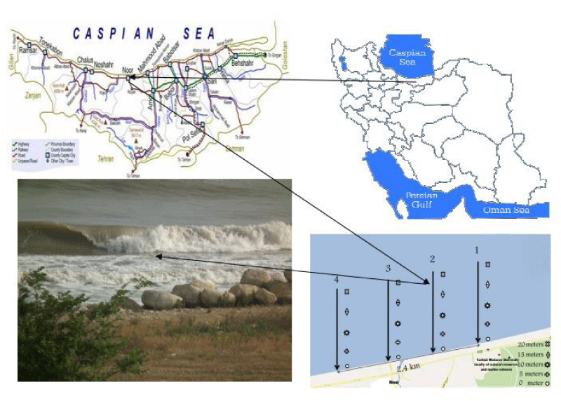
The segment of beach by 2.4 km in length at Noor’s coastal area, in the southern part of the Caspian Sea, in the North of Iran, was selected for this study. The beach is straight and open and lies between 36° 52’ 5.20” and 37° 17’ 40.93” N latitudes and 50° 32’ 17.16” and 53° 27’ 37.18” E longitudes. These measurements were carried out from September 2011 to June 2012. The mentioned stations were far apart 0.6 km in distance. The 0.6 km coastal stretch of Izadshahar City on the East and Royan City on the West forms the study area (Figure 1). Sediment samples were collected at 0 m, 5 m, and 10 m depths using grain size of the shoreline of the Caspian Sea.

Research method

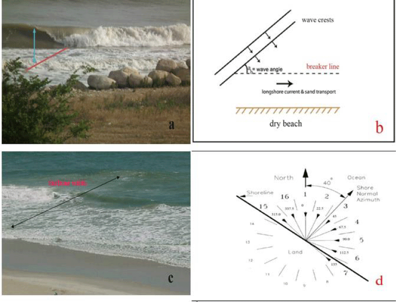
To carry out the present study, from September 2011 to July 2012, parameters including breaking wave height (H_b), wave period (T), breaking angle (a_b), surf zone width (W), using field observations at four stations, was measured and recorded (Figure 2). The oldest method used at present is to measure the buoyancy parameters (height, period of frequency, angle) and width of the coastal surfzone area. The measurement was conducted daily at four stations through the end of July 2012. For the measurement of the breakage wave heights, the foam was placed on the surface of the water tangent, and the distance between the surface and the corona to the fractured crown as a wave height of torture, which is shown in Figures 3-6 [33]. Then obtain the angle of the breaking wave height with the seaside, we observe the waves that are drawn off the coast from one conveyor that is close to the beach with eye observations [33]. In order to gain the period, the time interval between two successive waves was measured by the chronometer and the obtained value was recorded in the table. The distance between the first wave breakdowns to the coastal line was calculated to measure the width of the surfzone region using an eye monitor [33]. Samples from sediment across the zone, to analyze the sediment grain size distribution (d) on the coastline and in depths of 0 m, 5 m, and 10 m using a grapple, were taken and delivered to the laboratory. The alongshore current velocity in the surf zone (V) was measured by using a current meter and the bed slope was determined by dividing the water depth at a certain horizontal distance from the shoreline by this horizontal distance (Figure 2b).

The streamer trap method

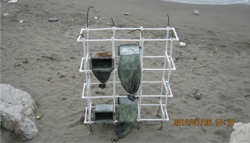
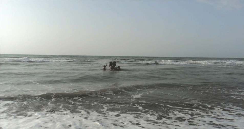
The device used in this study called the streamer trap used to measure the rate of sediment transport in the surfzone area. The name of the trapping device is captured from rectangular bags along with a sieve-type fabric, in which the flow is sediment and allows the water to cross over. The suspended trap was mainly designed to measure the rate of sediment transport in the coastal surfzone. And this debate is focused largely on it [34]. The rate of sediment transport along the beach can be measured using a suspended streamer trap. The used trap included a metal frame attached to the end of which are the bags of polyester monofilament sieve cloth, which was designed to capture the suspended sediments and bed. Trapping of sediment with traps is a natural method to measure the transport rate of point precipitation in the short term. It is possible to use a trap at the breakpoint area with waves less than two meters high and with one person to hold a trailer (Figure 3). A sieve cloth permits water to flow through but captures sediment particles of a nominal diameter greater than the mesh opening. Streamers in usage at CERC are made of 0.105 mm mesh cloth. In the United States, the cloth can be purchased in bolts 102 cm (40 in) wide and is bought per linear foot (30.5 cm) [35].

Trap design

The trapping framework is made of P.V.C. The rectangular section made of steel, which is connected to the tracker fabric, is made four centimeters on each side to be installed by bolts and beads on a stool to keep the trapping gap at high currents and throughout the flow distribution. Control factors include flow velocity along the beach, wave height, water depth, turbulence, grain size, and sampling time. On the other hand, the dependence of these factors on sampling time is still investigated. The height of the hanging trap is 1.2 m. Most sediment collected in traps is caused by flow. Traps are designed to prevent the removal of seditious materials and to ease the flow of water. However, the biggest problem is the trap around the bases during wave activity. Therefore, the presence of a person is required to hold a trap during sampling time. The bags are open, wrapped up, and closed by a Nayloni rope (Figure 3).

Trap operation

At the start of the cycle. The retention of the location of the marked area surfzone of the transfer, position of the traps involved, the way the openings of the traps involved flow along the coast located, and the base of the shelves for the perfect in the world, is also applied. Directly with the length of the trap wide as the crater flows into the Valley. If the weak current or alternating current, the entangled tend to spin around the basins, resulting in a fluctuation of water by the waves. Therefore, the action of tolerance against the downward currents and facing the trap beach is done by keeping the trap on the bed [36] (Figure 4).

Transport rate analysais

In this topic, a method for calculating the sediment transfer rate from raw data is explained. Such as moment samples, pumps, and audio sensor types, which are used to measure the sediment concentration, but the extract trap be used to extend sediment flux. For example, the weight of the sand is passing by the nozzle at a special cross-section of the sampling interval. If sampling was performed in a single-strain stream, the flux can be directly obtained with the developed flow by using the empirical formula of the predicted relative [36].

The flux of sand F at streamer k is given by:

$F\left(k\right)=\frac{s(k)}{△h△w△t}\text{ (1)}$

Where F is sand flux [kg. (m².s)^-1], k is the streamer number, raising in order from the bottom (k = 1) to the last streamer (k = N), S is the dry weight of sand (kg), ∆h is the height of streamer nozzle (0.15 m), ∆w is the width of streamer nozzle (0.25 m), ∆t is sampling time interval (s).

The flux between adjacent streamers, FE (k), can be predicted by linear interpolation using adjacent measured values:

$FE\left(k\right)=0.5[F\left(k\right)+F\left(k+1\right)]\text{ (2)}$

Alongshore Sediment Transport Rate (LSTR)

The LSTR is computed from the empirical equation reported by the alongshore energy flux in the breaker zone to the alongshore transport rate. The simplest and most commonly used methods for calculating LSTR are that of CERC [2,4,7,37] (Table 1).

In the above formulas, Q_s is the volume of alongshore transport rate in m³. (Year)^-1, H_b is breaking wave height in m, a_b is breaker angle with respect to the coastline, T_p is peak wave period in s, mb is beach slope near the breaking point, d50 is median grain size, K is dimensionless constant relating sand transport to longshore energy flux and was taken as 0.39, $A\text{ = }\frac{1}{\left[\left(\rho s-\rho \right)g\left(1-p\right)\right]},\rho s$ is the mass density of the sediment (2650 kg.(m^-3)), ρ is the mass density of seawater (1025 kg.(m^-3)), g is the acceleration due to gravity (9.81m.(s^-2)), p is the porosity of sediment (0.4), T is wave period in s, Cf is friction coefficient (0.005), W is surf zone width in m, V is measured alongshore current velocity (m.s-1), and $\left(\frac{\nu }{{\nu }_0}\right)LH$ is theoretical dimensionless longshore current velocity [36]. In the foregoing ratio, v_o is an initial alongshore current velocity and the index LH means mean level height wave [7].

Artificial Neural Network (ANN)

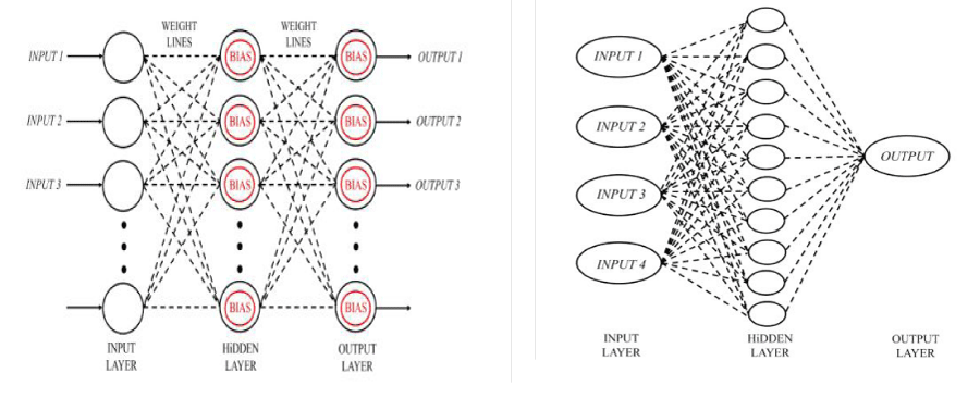
Concepts of ANN: ANNs are a relatively new non-linear statistical method that can be used to dissolve problems that are not suitable for conventional statistical methods. The ANNs are based on the present understanding of the biological nervous system, which includes some data processing sections called neurons or nodes that are grouped in layers. The input layer neurons get input data or information and send the values to the next layer of processing, getting across connections [38].

Figure 5 shows the basic artificial neuron. In this figure, diverse inputs to the network were demonstrated by the symbol x_n. Further input in the figure is named bias, θ, and it is always equivalent to one. Any of these inputs are multiplied together with a connection weight. These weights are demonstrated by w_n. In the simplest instance, these products are simply summed, fed through a transfer function, σ, to produce a result, and then output. In mathematical form, a neuron with n number of inputs is shown in Equation (3).

$Output=\sigma ({\sum }_{i=1}^n{w}_i\times x_i+\theta )\text{ (3)}$

Training of ANN: Distinguishing ANN weights is namely learning or training, and is equivalent to calibrating a mathematical model. The ANNs were trained by the input data and well-known output data. At the inception of training, the weights are Preliminary or with a random value or based on prior experiences. Then, the weights are systematically converted by the learning algorithm so that for a given input the difference between the ANN output and the observed output is lowered [38,40].

In the modeling process, the data sets of an alongshore current velocity, surf zone width, breaking wave height, and sediment transport rate were standardized to the range between 0 and 1, as follows:

$N_i= \frac{x_i-x_{min}}{x_{max}-x_{min}}\text{ (4)}$

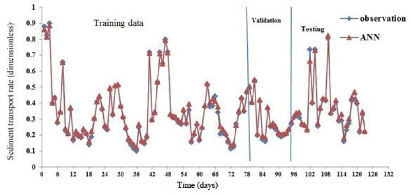
The structure of the neural network in this research, the three-layer network includes an input layer, a hidden layer, and an output layer. These types of networks are usually trained using the error-back propagation method. In order to prevent the weights of artificial neural networks from shrinking too much, the inputs of the network should be standardized. After standardizing the data, the number of network test data will be determined using the M test and the amount of gamma value. In the next step, the number of neurons in the input layer and the number of neurons in the hidden layer are determined. The artificial neural network model is trained using the training set and different combinations of inputs are made. In order to evaluate the results of the artificial neural network and compare them, the mean square error criterion, the efficiency coefficient, and the scatter diagram of the observational and estimated data are used. In order to prevent the weights of artificial neural networks from shrinking too much, we standardize the inputs of the network using the equation (4). X_n = normalized value, X_i = real value of variable, X_min = minimum real value of the variable and X_max = maximum real value of the variable. In this research, 70 percent of the data was used for training, 15 percent of the data was used for validation, and 15 percent was used for the test.

Performance evaluation: Four types of standard statistical criteria are proposed for statistical performance assessment. The root mean squared error (RMSE), efficiency coefficient (CE), mean absolute error (MAE), Scatter Index (SI), and mean relative error (MRE) was used. The RMSE is a good measure for evaluating the performance of a model because RMSE is proportional to the observed mean. Therefore, the SI forms a good non-dimensional error measure. The four performance evaluation criteria used in this study can be calculated utilizing Equations (5) to (10).

$RMSE=\sqrt{\frac{1}{n}{\displaystyle \sum }_{i=1}^n{(P_i-O_i)}^2}\text{ (5)}$

$CE=1-\frac{{{\displaystyle \sum }}_{i=1}^n{(O_i-P_i)}^2}{{{\displaystyle \sum }}_{i=1}^n{(O_i-{\stackrel{-}{O}}_m)}^2}\text{ (6)}$

$MAE=\frac{1}{n}|P_i-O_i|\text{ (7)}$

$MRE=\frac{1}{n}{\displaystyle \sum }_{i=1}^n\left|\frac{P_i-O_i}{{\stackrel{-}{O}}_m}\right|\times 100\text{ (8)}$

$SI=(\frac{RMSI}{Average observation value})\times 100\text{ (9)}$

$R^2=\frac{{{\displaystyle \sum }}_{i=0}^N(O_i-{\stackrel{-}{O}}_m)(P_i-{\stackrel{-}{P}}_m)}{{({{\displaystyle \sum }}_{i=1}^N{(O_i-{\stackrel{-}{O}}_m)}^2)}^{0.5}{({{\displaystyle \sum }}_{i=1}^N{(P_i-{\stackrel{-}{P}}_m)}^2)}^{0.5}}\text{ (10)}$

Where O_i and P_i are, respectively, the observed and predicted sediment transport rates, ${\overline{o}}_m$ is the average observed sediment transport rate and n is the number of observations. The RMSE is between zero and one, and the value of the error is as close as zero and shows the high accuracy of prediction. The index of scattering is regarding percentage and represents the percentage of scattering of the predicted data in comparison to the actual values, where the value of 0, represents a lack of scattering in the prediction. Moreover, the value of the correlation coefficient (R) between 1-1 and 1, and the value of 1, the predictor without errors. The domains are CE for infinity (weak model) up to 1 (good model) [32].

Results and discussion

Breaker characteristics

The daily alterations of breaking wave height, wave period, and breaker angle calculated from the wave measurements are shown in Table 2. The breaking wave height varied from 0.01m to 1.8 m with an average value of 0.47 m from September 2011 to June 2012. The wave period mostly varied from 1.91 to 7.4 s with a mean value of 4.65 s, and the mean wave-breaking angle was 27.80. The breaking waves approached the coast predominantly from the north (positive values). The mean surf zone width was about 84m. The daily statistical variables of wave characteristics [height (Hb), period (T) and angle (ab)], surf zone width (W), alongshore current velocity (V), beach slope (m), and grain size data (d) are shown in Table 2.

Sediment size distribution

The alterations from the middle size (d₅₀) and d₉₀ of the sediment at any trap location are shown in Table 3. As expected, d₅₀ increased from the water surface to the seabed at any trap location. In general, the sediments include fine sand (d₅₀ = 0.12 mm to 0.2 mm) to medium sand (d50 = 0.2 mm to 0.25 mm).

Alongshore sediment transport rates measured by streamer traps

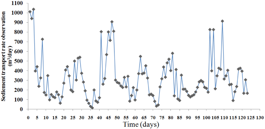
The sediment values observed by using the precipitation trapping method were evaluated daily between September 2011 and June 2012 on the coast of Noor. Then the sediment was transferred to the laboratory, and it was dried at 105 °C for 24 hours. Dried samples were weighed using digital scales. Then, the obtained values were placed in the formula. Values were plotted as 22 - 4 (Figure 6).

In Table 4, the final values of the sediment transfer rate in the Noor coastal area in the south of the Caspian Sea were calculated on an annual and daily basis.

Prediction of alongshore sediment transport rate

There were several methods for calculating the rate of sediment transport along the beach, which are the results of relations proposed for computing the rate of sediment transport. These differences are mainly due to the method upon which the equation has been obtained. Since these relations have been obtained for certain beaches, it is likely that the results of them on the coasts are not good ones. Therefore, before using these equations in each region we need to examine the constraints used. To determine the LSTR in the study area, long-term observations of shoreline changes and sediment properties, as well as measurement campaigns were performed. The LSTRs were obtained from three various methods [2,4,37].

According to the computer for the study area, the gross and the net LSTRs were obtained as shown in Table 5. The values of the statistical criteria for CERC, Walton and Bruno, and Kamphuis formulas are shown in Table 6.

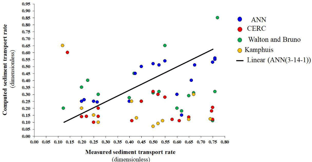
For the current study, the CERC formula used to be the most commonly applied expression in new models that contain more coastal parameters. It is recommended that the CERC formula is used in storm conditions where the wave heights overstep 4 m [5]. But, in the Noor coastal region, pursuant to the wave climate studies, the mean wave height was 0.3 m. Thus, the CERC equation overestimates LSTRs obtained from Kamphuis, Walton and Bruno, and ANN by factors of 0.97, 1.1, and 0.98, respectively. It is recommended to use Kamphuis’s formula in low-wave energy conditions with breaker heights of less than 1 m. The recommended value corresponds to the study area’s wave condition. Thus, Kamphuis’s equation overestimates LSTRs obtained from CERC, Walton and Bruno, and ANN by factors of 1.03, 1.14, and 1.01, respectively [2].

Application of ANN for prediction of LSTR

The data used in training the ANN model: Significant parameters in more sediment transport formulas are alongshore current velocity (V), surf zone width (W), and breaking wave height (H_b). In this study, observed data, obtained from the streamer trap, was used. Measured V, W, Hb values were used as input data to the model and sediment transport rate (Qs) as an output of the model. Generally, 123 samples are used for training the model, and 87 samples and 18 instances of total measured data, accidentally selected, were used for validation and testing the model.

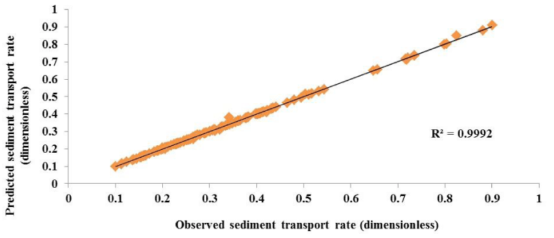
The alongshore transport rate is one of the most complex issues and many random variables affect its determination. This type of natural phenomenon is due to the conventional methods for estimating the rate of the parallel to the domain of change. In this research, the rate of sediment transport obtained from field observations and the Artificial Neural Network (ANN) model were evaluated and compared. According to the results of comparing the sediment transport rate observed and predicted by the ANN, the coefficient of regression coefficient (R2), root mean square error (RMSE), and Coefficient of Efficiency (CE) are 0.98, 0.02, 0.99, respectively, which indicates the effectiveness of the ANN model for estimation of sediment transport rate. The results confirm the superiority of artificial neural networks in the estimation of the parallel sediment transport rate of the coast, and in comparison of two activation functions, have confirmed the use of hyperbolic tangent function instead of sigmoid in predicting the sediment transport rate.

ANN model development: To select the foremost network for anticipation, various models are made by various nodes and medium layers. In the Learn Rate Control (LRC) feature, 0.001 and 0.15 were used as the minimum and maximum extent for auto control of the learning rate. The input compounds to estimate total sediment load are: 1) H, W, and V,2) Hand a_b; and 3) H_b, ab T, d50 and m. The first combination includes breaking wave height, alongshore current velocity, and surf zone width. The formula of Walton and Bruno is mostly used for the calculation of sediment transport rate. The other two compounds contain parameters used by CERC and Kamphuis formulas. Since try-and-error tests, the best network found in this study is the one with three layers containing one input layer, one middle layer, and one output layer. The best model consists of three input nodes including H_b, W and V, 14 middle nodes, and an output node, which must have a sigmoid transfer function. The sigmoid function indicative with 1/ (1+e^-x) sets the output single strength among 0 and 1. The correlation coefficient and RMSE of this model were 0.98 and 0.017 for the training data set and 0.96 and 0.015 for the test data set, respectively. The final architecture of the ANN model is given in Table 7.

The ANN model (3-14-1), which was trained using three main parameters of sediment transport rate rules, provides some rather accurate results into other models with four inputs. The precision of the selected ANN model (3-14-1) in comparison with other models of three inputs, particularly those with more than one hidden layer, has an insignificant difference. According to the complexity and longer time needed for the training of models with more than one hidden layer, the selection of the ANN model (3-14-1) is sensible. The comparison of the measured data and predicted whole sediment load using ANN for training and testing procedures is shown in Figure 7.

The scatterplot of the observed and predicted sediment transport rate of the ANN (3-14-1) model, in the validation period, is given in Figure 8.

The daily statistical variables of the breaking wave height (H_b), wave period (T), breaking wave angle (a_b), surf zone width (W), alongshore current (V), beach slope (m), grain size (d), sediment transport rate observation (Q₀), and sediment transport rate prediction (Q_ANN) are given in Table 8. In this table, S_x, CV and C_sx denote the standard deviation, variation, and skewness coefficients, respectively.

Comparison of the results of ANN and sediment transport rate formulas

123 sets of observed data with accurate wave properties, surf zone width, and alongshore current velocity data, not used in the training and validation of ANN in the prior section, were used to compare the results of the ANN model and sediment transport formulas. Field data including breaking wave height, wave period, breaking wave angle, surf zone width, alongshore current velocity, sediment particle size distribution, beach slope, and sediment transport rate, were measured by using a streamer trap.

In summary, the ANN model was trained using three significant parameters H_b, W, and V which can be further used to predict sediment transport rate in Caspian Sea data. However, the precision of an ANN model is data sensitive, and must not be practical to the situations outside the data range used in training the ANN model, without confirmation.

Figure 9 shows the predicted Q_S values compared with the observed Q_O values using CERC, Kamphuis, Walton and Bruno formulas, and the ANN method. The R², RMSE, CE, MRE, and MAE statistical criteria were used to calculate the results of the different models (Table 9).

Comparing the errors of this study with the error rate in the results of several international studies in the same field shows the accuracy of the results of this research. The results of some of these studies are as follows:

In Singh, et al. (2008) studies using a combination of network and nonlinear regression for the calculation of parallel shore transport rate, the coefficient of determination (R²), and the RMSE for data were 0.83 and 4.35 kg/s, respectively. Hashemi, et al. [19] at the Tormaduk coast of Ireland the seven-year period in 19 stations investigated the rate of the parallel sediment of the transport of the coast and compared the results with field data. The geometrical attributes of beach, wind, wave climate, and beach changes were considered. RMSE error was 0.0007. Using the Kabiri-Samani, et al. [8] approach, the wavelength, fragility wave angle, beach slope, and grain size as input and the sediment transport rate as output in a neural network, the values of coefficient of determination (R2) and RMSE were obtained equal to 0.6 and 0.6, respectively. A comparison of the errors of this research with international investigations indicates the high accuracy of the investigation shown in Table 10.

Conclusion

In this research, the rate of sediment transport was predicted and calculated using semi-experimental formulas and artificial neural networks in the Caspian Sea off the coast of the city of Noor. For this purpose, regional data was utilized by field observations (elevation, period, and angle), breakup surf zone width, grain size by sampling from Grab and determination of grain size in the laboratory by sieve shaker, velocity by using velocity meter and slope of the coast by using the mathematical formula of slope based on water depth and distance between the coastal lines, and the depth of scale of sediment The use of a trap has been measured and obtained.

Evaluating the accuracy of the empirical formulas and of the ANN was found to predict the rate of daily sediment transport. The LSTRs measured by the streamer sediment traps along the low-wave energy coast are lower than the rates estimated by the various empirical formulas. The generally used CERC formula, Kamphuis formula, and Walton and Bruno formula estimations were non-realistic high for the studied low-energy settings. The linear relationship between the energy flux factor and LSTR, included in the CERC formula, is supported by the streamer trap measurements. But, an order-of-extent lower empirical coefficient, 0.08 rather than 0.78, recommended by the Shore Protection Manual (1984), is proposed by the trap data for low-energy coast. Plus, studies on the comparability of the field techniques are recommended. Relationships among the different key measurements (Table 4) need to be explored to further understand their compatibility. ANN model is used for estimating sediment transport rate in the sea, in this study. 87 samples were used for training the ANN model and 36 samples were used to validate the model. Inputs for training the model include breaking wave height (Hb), surf zone width (W), and alongshore current (V). The results showed that the artificial neural network alongshore sediment transport rate in the Noor coastal zone can be calculated. The statistical criteria R2, RMSE, MAE, CE, and MRE for the ANN model, take the values 0.96, 0.015, 1.7 × 10^-4, 0.93, and 3.5 × 10^-2, respectively.

To achieve better results and complete the research path, it is recommended that the next sampling time should increase the observational migration rate in the future; To predict the rate of sediment transport, other models such as time series, regression, wavelet, fuzzy-neural inference system, and fuzzy logic has been used and the results have been compared with the results of the neural network.

1. Baktyar R, Dastgheib A, Roelvink D, Barry DA. Impacts of wave and tidal forcing on 3D nearshore processes on natural beaches. Part II: Sediment transport. Ocean Systems Engineering. 2016; 6:1; 61-97. https://doi.org/10.12989/ose.2016.6.1.061
2. Kamphuis JW. Alongshore sediment transport of sand. Journal of Waterway, Port, Coastal and Ocean Engineering, ASCE. 1991; 117:6; 624-641. https://doi.org/10.1061/(ASCE)0733-950X(1991)117:6(624).
3. Roushangar K, Shahnazi. Prediction of sediment transport rates in gravel-bed Rivers using Gaussian process regression. Journal of Hydroinformatics. 2020; 22(2): 249–262. https://doi.org/10.2166/hydro.2019.077.
4. US Army Coastal Engineering Research Centez. Shore Protection Manual, Department of the Army, Corps of Engineers, U.S. Govt. Printing Office, Washington, DC, USA, 1984; 1,2.
5. Sadeghifar T, Barati R. Application of adaptive Neuro-fuzzy inference system to estimate alongshore sediment transport rate (A real case study: southern shorelines of Caspian Sea). Journal of Soft Computing in Civil Engineering. 2018; 2-3:01-11. http://dx.doi.org/10.22115/SCCE.
6. Bakhtyar R, Yeganeh-Bakhtiary A, Ghaheri A. Application of neuro-fuzzy approach in prediction of run-up in swash zone. Applied Ocean Research. 2008; 30:17–27. https://doi.org/10.1016/j.apor.2008.02.004.
7. Bayram A, Larson M, Hanson H. A New Formula for the Total Longshore Sediment Transport Rate. Coastal Engineering. 2007; 54: 700-710. https://doi.org/10.1016/j.coastaleng.2007.04.001.
8. Kabiri-Samani AR, Aghaee-Tarazjani J, Borghei SM, Jeng DS. Application of Neural Network and Fuzzy Logic Models to Long-shore Sediment Transport. Applied Soft Computing. 2011; 11: 2880-2887. https://doi.org/10.1016/j.asoc.2010.11.021.
9. Adnan RM, Sadeghifar T, Alizamir M, Torabi Azad M, Makarynsky O, Kisi O, Barati R, Ahmed KO. Short-term probabilistic prediction of significant wave height using Bayesian model averaging: Case study of Chabahar port, Iran. Ocean Engineering. 2023; 272(113887).
10. Kalra R, Deo MC, Kumar R, Agarwal VK. Artificial neural network to translate offshore satellite wave data to coastal locations. Ocean Engineering. 2005; 32:1917–1932. https://doi.org/10.1016/j.oceaneng.2005.01.007.
11. Lee KH, Mizutani N, Kim DS, Fujii T. Estimation of wave breaking in gravel beach using artificial neural network. In: Proceedings of the International Offshore and Polar Engineering Conference. 2009; 951–957.
12. Pape L, Ruessink BG, Wiering MA, Turner IL. Recurrent neural network modeling of nearshore sandbar behavior. Neural Netw. 2007 May;20(4):509-18. doi: 10.1016/j.neunet.2007.04.007. Epub 2007 Apr 29. PMID: 17532608.
13. Yan B, Zhang QH, Wai OWH. Predictions of sand ripple geometry under waves using an artificial neural network. Computers and Géosciences. 2008; 34:1655–1664. https://doi.org/10.1016/j.cageo.2008.03.002.
14. Ghorbani MA, Khatibi R, Aytek A, Makarynskyy O, Shiri J. Sea water level forecasting using genetic programming and comparing the performance with artificial neural networks. Computers and Geosciences. 2010; 36(5): 620–627. https://doi.org/10.1016/j.cageo.2009.09.014
15. Huang W, Murray C, Kraus N, Rosati J. Development of a regional neural network for coastal water level predictions. Ocean Engineering. 2003; 30:2275–2295. https://doi.org/10.1016/S0029-8018(03)00083-0.
16. Lee TL, Makarynskyy O, Shao CC. A combined harmonic analysis—artificial neural network methodology for tidal predictions. Journal of Coastal Research. 2007; 23(3):764-770.https://doi.org/10.2112/05-0492.1.
17. Makarynska D, Makarynskyy O. Predicting sea level variations at the Cocos (Keeling) Islands with artificial neural networks. Computers and Geosciences. 2008; 34(12):1910–1917. https://doi.org/10.1016/j.cageo.2007.12.004/.
18. Browne M, Castelle B, Strauss D, Tomlinson R, Blumenstein M, Lane C. Near-shore swells estimation from a global wind–wave model: spectral process, linear, and artificial neural network models. Coastal Engineering. 2007; 54:445–460. https://doi.org/10.1016/j.coastaleng.2006.11.007.
19. Iglesias G, Lopez I, Carballo R, Castro A. Headland-bay beach plan form and tidal range: a neural network model. Geomorphology. 2009; 112:135–143. https://doi.org/10.1016/j.geomorph.2009.05.014.
20. Liang SX, Li MC, Sun ZC. Prediction models for tidal level including strong meteorologic effects using a neural network. Ocean Engineering. 2008; 35:666–675. https://doi.org/10.1016/j.oceaneng.2007.12.006.
21. Panizzo A, Briganti R. Analysis of wave transmission behind low-crested breakwaters using neural networks. Coastal Engineering. 2007; 54:643–656. https://doi.org/10.1016/j.coastaleng.2007.01.001.
22. Yagci O, Mercan DE, Cigizoglu HK, Kabdasli MS. Artificial intelligence methods in breakwater damage ratio estimation. Ocean Engineering. 2005; 32:2088–2106. https://doi.org/10.1016/j.oceaneng.2005.03.004.
23. Teodoro AC, Veloso-Gomes F, Gonc-Alves H. Retrieving TSM concentration from multispectral satellite data by multiple regression and artificial neural networks. IEEE Transactions on Geoscience and Remote Sensing. 2007; 45:1342–1350. DOI: 10.1109/TGRS.2007.893566.
24. Hashemi MR, Ghadampour Z, Neill SP. Using an Artificial Neural Network to Model Seasonal Changes in Beach Profiles. Ocean Engineering. 2010; 37:1345-1356. https://doi.org/10.1016/j.oceaneng.2010.07.004.
25. Boveriri HR, Musddad SM. Sedimentation Rate in Waters around Iran. International Journal of Research in Management. 2012; 2(2): 239-246.
26. Malekmohamadi I, Ghiassia R, Yazdanpanah MJ. Wave hindcasting by coupling numerical model and artificial neural networks. Ocean Engineering. 2008; 35:417–425. https://doi.org/10.1016/j.oceaneng.2007.09.003
27. Londhe SN, Panchang V. One-day wave forecasts based on artificial neural networks. J. Atmos. Oceanic Tech- nol. 2016; 23:1593–1603. https://doi.org/10.1175/JTECH1932.1
28. Deshmukh AN, Deo MC, Bhaskaran PK, Balakrishnan Nair TM, Sandhya KG. Neural-network- based data assimilation to improve numerical ocean wave forecast. IEEE J. Oceanic Eng. 2016; 41:944–953. https://doi.org/10.1109/JOE.2016.2521222.
29. Sadeghifar T, Motlagh MN, Azad MT, Mahdizadeh MM. Coastal wave height prediction using Recurrent Neural Networks (RNNs) in the South Caspian Sea. Marine Geodesy. 2017; 40:2; 454-465. https://doi.org/10.1080/01490419.2017.1359220.
30. Elbisy MS, Osra FA. Application of Group Method of Data Handling Type Neural Network for Significant Wave Height Prediction.American Journal of Neural Networks and Applications. 2019; 5 (2):51-57. doi: 10.11648/j.ajnna.20190502.12.
31. Cannas B, Fanni A, See L, Sias G. Data preprocessing for river flow forecasting using neural networks: wavelet transforms and data partitioning. Phys. Chem. Earth, Parts A/B/C. 2006; 31 (18): 1164–1171.https://doi.org/10.1016/j.pce.2006.03.020.
32. Ozger M. Significant wave height forecasting using wavelet fuzzy logic approach. Ocean Engineering. 2010; 37(16):1443–1451. https://doi.org/10.1016/j.oceaneng.2010.07.009.
33. Thomas LJ, Seabergh WC. Littoral Environment Observations. U.S. Army Engineering Waterways Experiment. Station. Coastal Engineering Research Center 3909 Halls Feny Road, Viiurg. Missiiippi. 1997; 39180-6lS9.
34. Bodge KR, Kraus NC. Critical examination of long-shore transport rate amplitude. Proceedings of Coastal Sediments 1991, ASCE, New York. 1991; 139-155.
35. Brinkkemper JA, Aagaard T, de Bakker ATM, Ruessink BG. Shortwave Sand Transport in the Shallow Surf Zone. J Geophys Res Earth Surf. 2018 May;123(5):1145-1159. doi: 10.1029/2017JF004425. Epub 2018 May 28. PMID: 30034978; PMCID: PMC6049877.
36. Leenknecht DA, Szuwalski A, Sherlock AR. Automated Coastal Engineering System- User's Guide. Technical Report, US Army Corps of Engineers, Waterways Experiment Station, Coastal Engineering Research Center, Vicksburg, Mississippi. 1992.
37. Walton Jr TL, Bruno RO. Longshore transport at a detached breakwater, phase II. Journal of Coastal Research. 1989; 65(9): 667– 668.
38. Mostafa RR, Kisi O, Adnan RM, Sadeghifar T, Kuriqi A. Modeling Potential Evapotranspiration by Improved Machine Learning Methods Using Limited Climatic Data. Water. 2023; 15:486.
39. Sadeghifar T, Lama GFC, Sihag P, Bayram A, Kisi O. Wave height predictions on complex sea flows through soft-computing models: Case study of Persian Gulf, Ocean Engineering. 2022; 245: 110467. https://doi.org/10.1016/j.oceaneng.2021.110467.
40. Ikram RMA, Cao X, Sadeghifar T, Kuriqi A, Kisi O, Shahid S. Improving Significant Wave Height Prediction Using a Neuro-Fuzzy Approach and Marine Predators Algorithm. J. Mar. Sci. Eng. 2023; 11:1163. https://doi.org/10.3390/jmse11061163.