A Numerical Case Study of the Impact of Submesoscale Feedbacks on Mesoscale Eddies

2.1. High-resolution model simulation

The Regional Oceanic Modeling System (ROMS) is employed, and it has been widely applied to oceanic multiscale dynamical research [1,24,39-42]. As shown in Figure 1, the parent D0 domain covers the Northwest Pacific STCC ranging from 110°E-165°E to 12°N-28°N with a relatively low horizontal resolution of 9km. Then, an online two-way nesting is adopted for child D1 and D2 domains with successive resolution refinement from 3km to 1km. The child D1 domain has 677×257 orthogonal grid points from 123° to 144°E and 15.5° to 23.5°N, covering the core region where mesoscales are most frequently generated [11]. The refined child D2 domain has 548×506 orthogonal grid points from 136°°E to 141.5°E and 17.5°°N to 22.5°N, covering a typical mesoscale dipole of cold-warm eddies in the simulation.

Figure 1: a) An illustration of the parent (D0) and child domains (D1 and D2). The shown is a snapshot of the surface Rossby number $$Ro=\zeta /f$$ , the ratio of vertical relative vorticity ζ to the local Coriolis parameter f) with 0.00 feedback coefficient α in different domains on 20 May 2018. The parent D0 domain has a horizontal resolution of 9 km and two boxes inside denote the successive nesting child D1 domains of 3km and D2 1km resolutions, respectively. b) Schematic diagram of the modified downscaling scheme with controllable feedback strength for child D1 and D2 domains. The black dotted lines in child D1 domain denote the feedback area where the controllable two-way nesting is implemented. xfine and xcoarse indicates the variables in child D1 and D2 domains. The filling variable is the surface R0 on 20 May 2018 with 0.00 feedback coefficient.

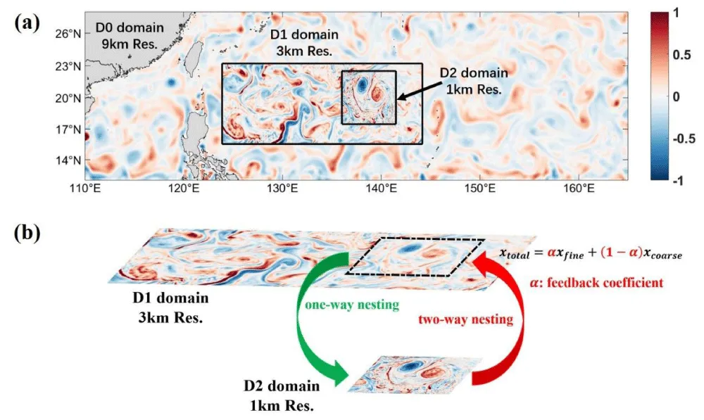
Vertically, all three domains consist of identical 60 layers with concentrated levels in the upper ocean. The bathymetry is linearly interpolated from the GEBCO 2023 dataset and slightly smoothed to avoid exceeding computational restrictions of topography steepness and roughness [43]. The surface atmospheric forcings, including heat fluxes and wind stress, are derived from hourly CFSv2 reanalysis data with a spatial resolution of 1/4°. The oceanic lateral boundary and initial conditions driving the parent D0 domain are interpolated from the daily 1/12° HYCOM dataset, and the K-profile parameterization is employed for the vertical turbulence closure scheme [44]. The tidal model is not included in the simulation.

The parent D0 domain is configured for spin-up to satisfy dynamics and thermodynamics consistency, and then provides initial and daily lateral boundaries for the following two-way nesting. After a 15-month simulation from January 2017 to March 2018, the parent D0 domain achieves numerical equilibrium within the upper 500m and then runs an additional 3 months to provide daily-averaged boundaries for the child D1 domain from April to June 2018. The model outputs, including large-scale current, thermohaline structure, mixed layer depth (MLD), and mesoscale KE level, are validated against satellite observations and reanalysis datasets before downscaling. Subsequently, the nesting of child D1 and D2 domains runs from April to June in 2018 under the same surface atmospheric forcings. The time steps for child D1 and D2 domains are set to 60s and 20s, respectively. Both domains provide outputs of hourly snapshots. Particularly, a mesoscale dipole of cold-warm eddies occurs during the simulation shown in figures 1-4, and we attempt to explore the impact of submesoscale feedback on mesoscales using a modified two-way nesting framework.

Figure 3: Same as Figure 2 but for the date of 04 Jun 2018.

Figure 4: The mean horizontal wavenumber spectra of KE in the feedback area D2 with different feedback coefficients (0.00, 0.25, 0.50, 0.75 and 1.00) and the “Truth” at the depths of a) 10m and b) 200m from May 20 - June 09, 2018. Straight black and blue dotted lines show spectral slopes of K-2) (surface quasi-geostrophic theory) and K-3) (interior quasi-geostrophic theory), where K is the isotropic wavenumber.

Figure 5: The frequency-wavenumber spectra of KE in the feedback area D2 with different feedback coefficients (0.00 to 1.00 in a-e) and the “Truth” f) at the depth of 10m from May 20 - June 09, 2018. Three straight black dotted vertical lines indicate the spatial scale of 50 km, 10 km and 5 km (0.02, 0.1 and 02 cpkm), respectively. The straight horizontal white solid line shows the inertial frequency f. Note that the colorbar uses a logarithmic scaling to base 10.

2.2. A downscaling scheme of two-way nesting with controllable feedback strength

There are two categories of online nesting frameworks, termed one-way and two-way in ROMS [45,46]. In one-way nesting, the coarser domain only provides lateral boundaries for the finer domain by spatial and temporal interpolations at each nesting coupling time step. Nevertheless, in two-way nesting, besides the above one-way nesting procedures, the finer domain also feeds back spatial-averaged fluxes to the corresponding coarser grid points within the feedback area (marked by black dotted lines in Figure 1b). While one-way nesting has been widely applied in previous downscaling studies (e.g. [1,35]), two-way nesting can be designed to detect multiscale interactions. Here, the two-way nesting is slightly modified by introducing a feedback coefficient a that controls the fluxes proportion from the finer to coarser domain (shown in Figure 1b),

$$\begin{array}{c}{x}_{total}=\alpha x_{fine}+\left(1-\alpha \right)x_{coarse},\end{array}\text{ (1)}$$

Where a is the feedback coefficient from 0 to 1, and x_fine  is the spatial-averaging fluxes from finer D2 to coarser D1 domain, x_coarse  is the fluxes in the coarser D1 domain. To systematically evaluate the impact of submesoscale feedback on mesoscales, we implement five cases with different feedback coefficients ranging from 0.00 to 1.00 with an interval of 0.25. When the value of a is 1.00, all variables within the feedback area (finer-gridded D2) within the coarser D1 domain are replaced by the spatially-averaged finer D2 variables at each grid and each nesting coupling time. Conversely, if the value of a is 0.00, it means no finer D2 domain fluxes feed back to the coarser D1 domain, which downgrades to the one-way nesting. In this study, each coarser-grid point (in 3 km-resolution D1 domain) covers nine finer-grid points (in 1 km-resolution D2 domain), and the finer D2 domain returns fluxes to the coarser D1 domain every 3 steps (60s) at the coarser domain integration time. Furthermore, an experiment with 1 km horizontal resolution in the whole D1 domain is performed to establish a “Truth” simulation. Then, the degree to which the results in the feedback area with different feedback strength (controlled by the coefficient a) approach the “Truth” serves as an assessment of the impact of submesoscale feedbacks on mesoscales. Physically, a represents the efficiency with which explicitly resolved submesoscale processes (e.g., mixed-layer instabilities) feed back onto the mesoscale flow.

2.3. Spectral approach

The spectral approach is employed to compute the wavenumber and frequency-wavenumber spectra in this study. Here, we follow the preprocessing of Schubert, et al. [35]. Before the use of fast Fourier transformation, the outputs within the feedback area are first transformed from the geographical into Cartesian coordinates, and linearly interpolated onto a regular 1km grid spacing, considering the horizontal resolution of the finer D2 domain is 1km. Then, the variables are partitioned into 4 overlapping square boxes with a length of 256 km [32], which are large enough to capture the impact of submesoscale feedback on mesoscales. After removing the best-fit two-dimensional spatial slopes and applying a 2D Hanning window, the Fourier transformation is utilized to transition from physical to spectral space before multiplying an associated amplitude correction factor of 1.5 [35]. The Fourier transformation of a 2D horizontal field F(x,y) is defined as,

$$\begin{array}{c}\hat{F}\left(k,l\right)=\frac{1}{{\left(2\pi \right)}^2}{\displaystyle {\int }_{-\infty }^{\infty }}{\displaystyle {\int }_{-\infty }^{\infty }}F\left(x, y\right)e^{-i\left(kx+ly\right)}dxdy, \end{array}\text{ (1)}$$

of which k and l are the zonal and meridional wavenumber components, respectively. For example, the cumulative power spectral density of KE associated with horizontal velocities u, v is derived as,

$$\begin{array}{c}E\left(K\right)=\frac{1}{N^2}{\displaystyle {\int }_0^K}\frac{1}{2}\left({\widehat{u}}^{*}\widehat{u}+{\widehat{v}}^{*}\widehat{v}\right)dK, \end{array}\text{ (2)}$$

Where N is the number of square box points along each side, and the power spectral density is normalized by the area $$N^2.\text{}\text{}\text{}K=\sqrt{k^2+l^2}$$ is the isotropic wavenumber and * denotes the complex conjugate. Then, the 1D wavenumber spectra of KE are given by 2p(dE/dK).

The computation process for frequency-wavenumber spectra is essentially the same, with the only difference being the addition of the time dimension. The details of deriving the spectra can be found in Cao, et al. [47].

2.4. Coarse-graining approach

We further employ the coarse-graining approach to quantitatively evaluate the scale kinetic energy flux. This approach has been earlier introduced to turbulence problems by Leonard [48], and then applied to oceanic multiscale dynamics recently [35,49,50]. It’s advantageous to traditional methods due to no assumption of homogeneous and isotropic turbulence and free of windowing [35]. Specifically, this method can be regarded as a “blurring” process [51], which is achieved mathematically by applying a low‐pass filter with a convolution method.

A horizontal field F(x, y) is low-pass filtered by applying a convolution $$\stackrel{-}{F}\left(x, y\right)=C\times F(x, y)$$ with a top-hat kernel [35],

$$\begin{array}{c}C\left(r\right)=\{\begin{array}{c}1/A, if \left|r\right|<L/2,\\ 0, otherwise,\end{array}\end{array}\text{ (3)}$$

Where A = πL²/4 is the area of a circle with diameter L and r is the radial vector. The expression for the horizontal scale kinetic energy flux across scale l, Π _l (x) can be obtained when applied to the dynamical equations [50],

$$\begin{array}{c}{\Pi }_l\left(x\right)=-{\rho }_0\left[\left(\overline{u_l^2}-{\overline{u}}_l^2\right){\overline{u}}_{l_x}+\left(\overline{u_l{v}_l}-\overline{u_l}\overline{v_l}\right)\left({\overline{u}}_{l_y}+{\overline{v}}_{l_x}\right)+\left(\overline{v_l^2}-{\overline{v}}_l^2\right){\overline{v}}_{l_y}\right],\end{array}\text{ (4)}$$

of which a negative (positive) value of Πl (x) indicates horizontal KE transfers directed toward a larger (smaller) scale than l. In this paper, Πl (x) is computed in the following length scales of 4, 8, 10, 16, 20, 24, 30, 34, 40, 44, 50, 60, 70, 80, 90, 100, 120, 140, 160, 180, and 200 km.

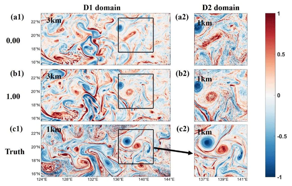
Figure 2 shows the surface Rossby number (, $$Ro=\zeta /f$$ the ratio of vertical relative vorticity $$\zeta$$ to the local Coriolis parameter f) in three cases of 0.00, 1.00 feedback coefficients, and the “Truth” on 20 May 2018. Overall, it exhibits active mesoscales in both D1 and D2 domains. Moreover, the “Truth” in figure 2c1 shows more abundant submesoscales than that in figure 2a and 2b, verifying that the improvement of horizontal resolution from 3 km to 1 km can remarkably resolve more submesoscales. Compared with the feedback area marked by a solid black line in figure 2a1 and 2b1, submesoscales with a 1.00 feedback coefficient are more intense than those with a 0.00 feedback coefficient, suggesting that the D1 domain can absorb more refined submesoscales resolved by the D2 domain through consecutive flux exchanges in two-way nesting. figure 2a2 and 2b2 of the D2 domain both reveal more abundant and detailed submesoscale fronts and tail-shaped filaments in the periphery of mesoscales than those in figure 2a1 and 2b1. Additionally, the spatial patterns in figure 2a2 and 2b2 exhibit a similar mesoscale dipole structure to the “Truth” in figure 2c2 except that they are much noisier.

Figure 2: Snapshots of surface Rossby number (Ro=ζ/f) on 20 May 2018. a1-b1) The results of D1 domain with 0.00 and 1.00 feedback coefficients as the interior small domain D2 is downsaled to 1 km resolution. c1) The “Truth” referred for panels a) and b), which is the simulation result of 1km resolution in the entire domain D1. The solid black box in panels a1-c1 denotes the downscaled domain D2 that makes detailed information feedbacked to D1. a2-c2) The enlarged version of small domain D2 denoted by the solid black boxes in panels a1-c1, respectively.

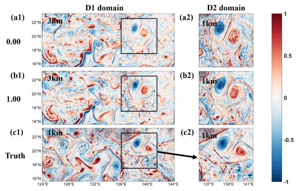
However, the cyclonic eddy in the mesoscale dipole displayed noteworthy morphological differences among the three cases on 04 Jun 2018. As shown in figure 3a1, it is significantly elongated in the case with 0.00 feedback coefficient, while the deformation is negligible and remains basically circular shape in both the cases of 1.00 feedback coefficient (figure 3b1) and the “Truth” (figure 3c1). Considering the use of an identical model configuration as well as oceanic and atmospheric forcing, the only reason causing this morphological deformation is the feedback strength. That is, if the finer D2 domain provides submesoscale feedback to the coarser D1 domain, the cyclonic eddy in the mesoscale dipole behaves more coherently and is not sensitive to deformation. Conversely, if there’s no feedback, the cyclonic eddy is loose and more prone to being stretched. However, the other anticyclonic eddy exhibits almost no morphological difference except for the geographical location.

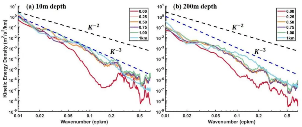
To evaluate the impact of submesoscales feedback on the maintenance of the cyclonic eddy in this study, the mean horizontal wavenumber spectra of KE in the feedback area with different feedback coefficients and the “Truth” are displayed in figure 4. In the mesoscales range of about 50 and 100 km (0.01-0.02 cpkm), all spectra slopes drop close to the interior quasi-geostrophic theory of K-3 in both the upper (10m) and interior (200m) ocean [52,53]. Meanwhile, the magnitude of KE in cases with 0.25 to 1.00 feedback coefficients is significantly strengthened compared to that with a 0.00 feedback coefficient, which is consistent with previous findings that mesoscales can be strengthened by submesoscale KE to make them more coherent and not quickly dissipated with a KE increase [36]. This partially explains the persistence of the cyclonic eddy in the mesoscale dipole.

However, the KE spectra display significant differences at scales below 50 km (0.02 cpkm). In the upper ocean of 10 m depth, the spectra with 0.00 feedback coefficient continue to drop with a slope of about K-3 down to 15 km (about 0.06 cpkm), below which it decreases sharply due to the dominant effect of model dissipation [35]. We may define the effective resolution as the wavelength at which the kinetic energy spectrum begins to deviate significantly from the theoretical slope K2. Thus, a scale of 15 km can be identified as the effective resolution of the D1 domain (it requires at least 4-6 grid spacings to resolve an eddy in a model). While the cases with 0.25 to 1.00 feedback coefficients and the “Truth” follow a shallower slope close to the predictions of surface quasi-geostrophic theory K-2 between 15 km and 50 km (0.02-0.06 cpkm) [54,55]. This further confirms that the enhancement of horizontal resolution from 3 km to 1 km can significantly improve the capability to resolve more submesoscales. According to theoretical analysis, Dong [56] estimates the Mixed Layer Instability (MLI) sinusoidal wavelength globally and indicates that it is smallest in summer when using the KPP vertical turbulence closure scheme. The corresponding bound of the MLI sinusoidal wavelength is approximately 10 km within the feedback area during the simulation period [57]. Therefore, the improvement of horizontal resolution from 3 km to 1 km can effectively resolve the MLI, directly improving the ability to capture more submesoscales [56]. Similarly, the “Truth” declines sharply at a scale of approximately 5 km (0.2 cpkm). That suggests that the effective resolution of the D2 domain can be 5 km. Furthermore, it’s noteworthy that the KE in cases with feedback coefficients of 0.25 to 1.00 is significantly larger than that with a 0.00 feedback coefficient, which is very close to the “Truth” whose magnitude is largest. This suggests that the D2 finer domain can transmit smaller and more detailed submesoscales to the D1 coarser domain through high-frequency flux exchanges in two-way nesting. Nevertheless, the magnitude of KE exhibits almost no difference among cases with 0.25 to 1.00 feedback coefficients, which indicates that the submesoscales are insensitive to the feedback strength. Additionally, the KE with feedback coefficients of 0.25 to 1.00 shows the largest value below the D2 domain effective resolution of 5 km; this may be attributed to the numerical error associated with mathematical interpolation in preprocessing, but it is out of the scope of physics.

The KE at 200 m depth is approximately an order of magnitude smaller than that at 10 m depth. Although previous studies indicate that submesoscales are mainly concentrated within the upper mixed layer [16,21,24,34,58], the spectral slopes in cases with 0.25 to 1.00 feedback coefficients and the “Truth” still approach the predictions of surface quasi-geostrophic theoryK-2between 15 km and 50 km (0.02-0.06 cpkm). This dynamical characteristic is also observed in the eastern tropical Pacific Ocean [59]. Meanwhile, the remarkable improvements of KE between 15 km and 50 km further validate that the finer D2 domain can resolve smaller-scale dynamics and fuel the coarser D1 domain through consecutive flux exchanges in the two-way nesting even at the depths of 200 m. Below 15km, the spectra in cases with 0.00 to 1.00 become much noisier, which is related to the mathematical interpolation numerical error.

As a summary, in the experiment with 0.0 feedback coefficients for a 3km resolution grid, the spectrum rolls off at about 0.06 cpkm (about ~15 km) wavelength, indicating an effective resolution of only ~15 km. In the “Truth” of 1km grid resolution, the spectrum maintains the theoretical slope down to 0.2cpkm (~5 km), demonstrating that submesoscale feedback improves the effective resolution to ~5 km.

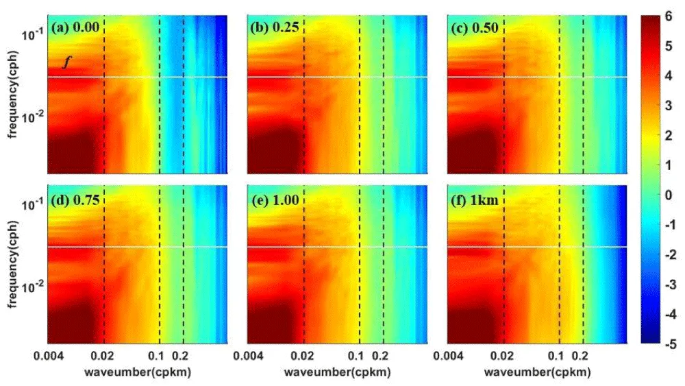
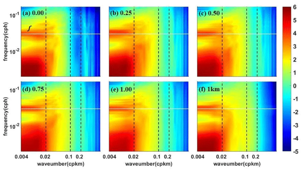
The frequency-wavenumber spectra of KE in the feedback area with different feedback coefficients and the “Truth” at 10m depth are displayed in figure 5. As shown, the magnitude of KE monotonically decreases from larger, slower to smaller, quicker scales along both the wavenumber and frequency axis [60]. This is consistent with the 1D horizontal wavenumber spectra, as the submesoscale KE is orders of magnitude smaller than mesoscales. Although the frequency-wavenumber spectra reveal broadly similar patterns, significant differences are evident in the details. Within the spatial scale range of 5 km (0.2 cpkm, the effective resolution of D2 domain) to 50 km (0.02 cpkm, about upper bound of submesoscales), the magnitude of KE with 0.25 to 1.00 feedback coefficients is significantly larger than that with 0.00 feedback coefficient though it remains lower than the “Truth”, particularly between 5km to 10km (0.1 to 0.2 cpkm, marked by black dotted line in figure 5). This further confirms that the coarser D1 domain is capable of absorbing the refined submesoscales resolved by the finer D2 domain in two-way nesting.

As illustrated in figure 6, while the magnitude of KE significantly decreases at a depth of 200m, the frequency-wavenumber spectra of KE exhibit similar patterns to those at 10m depth. In the scale range below 50 km (0.02 cpkm), the KE in cases with 0.25 to 1.00 feedback coefficients is greater than that with 0.00 feedback coefficient, which is also clearly demonstrated in the 1D wavenumber spectra in figure 4. This phenomenon is particularly pronounced at smaller scales of about 5 km to 10 km, where the KE is at least an order of magnitude larger than that with 0.00 feedback coefficient. This further indicates that the coarser D1 domain is capable of capturing much smaller and more refined dynamical processes that can be directly resolved by the finer D2 domain, even though the submesoscales are extremely weak at a depth of 200 meters underwater. Meanwhile, there is little difference among the cases with 0.25 to 1.00 feedback coefficients, further indicating that the energy level is largely insensitive to the feedback strength in the modified two-way nesting. Meanwhile, in the deep ocean, inertia-gravity waves become significant and manifest as energized wave banded regions within the KE frequency-wavenumber spectra KE, where the dispersion relations of free, linear inertia-gravity waves are located [61]. Figure 6 shows a weak but distinct banded signature of inertia-gravity waves in the high-frequency, low-wavenumber region near the inertial frequency f. However, the gravity wave signal is not apparent within the upper ocean of 10m in Figure 5 [60].

Figure 6: Same as Figure 5 but at the depth of 200 m. The colorbar uses a logarithmic scaling to base 10.

Figure 7: Same as Figure 5 but for the normalized vertical relative vorticity (ζ/f, a1-f1) and horizontal divergence (Div/f, a2-f2).

Figure 8: Same as Figure 7 but at the depth of 200m.

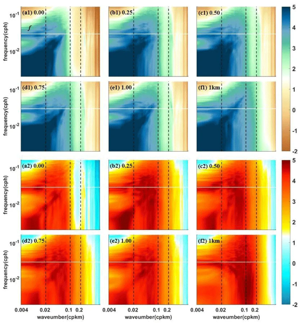
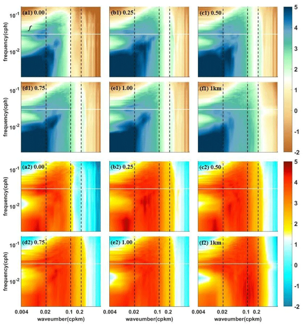
According to previous studies [47,61,62], submesoscales display significant rotational and divergent dynamical characteristics, which can be reflected in the frequency-wavenumber spectra of normalized vertical relative vorticity $$\zeta /f=(v_x-u_y)/f$$ and horizontal divergence ( $$Div/f=(u_x+v_y)/f$$ ) by inertial frequency f [60]. To better demonstrate the impact of submesoscales feedback on mesoscales with different feedback coefficients, we present the frequency-wavenumber spectra of $$\zeta /f$$ (a1-f1) and $$Div/f$$ (a2-f2) in the feedback area at the depth of 10m in figure 7. Different from the frequency-wavenumber spectra of KE depicted in figure 5, the large value of $$\zeta /f$$ can extend down to submesoscales range of about 10 km (0.1 cpkm). Dynamically, submesoscales are characterized by an increase of vertical relative vorticity, indicating that they are marginally constrained by the Earth’s rotation [27,50]. Since the effective resolution of the “Truth” is about 5 km, it can resolve more refined submesoscales than other cases and demonstrate significantly enlarged values in the smaller-scale submesoscales range of approximately 5km to 10km (0.1 to 0.2 cpkm). While the effective resolution in the case of 0.0 feedback coefficient is only about 15 km, the model can’t directly resolve dynamical processes smaller than this scale. Instead, these smaller processes are represented by parameterization in the simulation, which merely serves as a rough approximation and significantly underestimates their intensity. Consequently, the magnitude of $$\zeta /f$$ in the range of 5 km to 15 km with 0.00 feedback coefficient is so weak that it is nearly negligible. Nevertheless, the $$\zeta /f$$ in cases with 0.25 to 1.00 feedback coefficients reveal significant improvements due to flux exchanges in two-way nesting, even though they remain lower than the “Truth”. This further validates that the coarser D1 domain can partially absorb smaller-scale submesoscales that can’t be directly resolved by itself from the finer D2 domain.

Different from the vertical relative vorticity $$\zeta /f$$ , the frequency-wavenumber spectra of horizontal divergence $$Div/f$$ predominantly reach their maximum at wavelengths within the submesoscales range. This phenomenon has also been highlighted by Cao [60], who differentiates mesoscales and submesoscales based on the characteristics of $$\zeta /f$$ and $$Div/f$$ frequency-wavenumber spectra. Dynamically, submesoscales are also characterized by a remarkable improvement of horizontal divergence resulting from the enlarged ageostrophic vertical transport, which can induce considerable convergence and divergence within submesoscale zones. Similarly, the magnitudes of $$Div/f$$ with 0.25 to 1.00 feedback coefficients are significantly improved compared to those with 0.00 feedback coefficient. Additionally, it is noteworthy that the peak of $$Div/f$$ tends to shift towards smaller wavelengths as the horizontal resolution increases, which is evident in cases with 0.00, 1.00 feedback coefficients and the “Truth” in figure 7a2, 7e2 and 7f2. We will further confirm in the subsequent snapshots of Div in figure 14b1-14b6, as the horizontal resolution increases, the spatial scale of Div indeed decreases progressively.

Compared to the upper ocean, the magnitude of $$\zeta /f$$ and $$Div/f$$ in frequency-wavenumber spectra at 200m depth are both dramatically reduced in the submesoscale range of about 5 km to 50 km (0.02 to 0.2 cpkm). Concurrently, mesoscale horizontal divergence also exhibits a remarkable decline, whereas the vertical relative vorticity within the mesoscales (0.004 to 0.02 cpkm) remains relatively large, which suggests the presence of energetic mesoscale effects accompanied by weakened submesoscale dynamics in the deep ocean [60]. Cao [60] also suggests that energetic submesoscale divergence mainly originates from the turbulent cascades of submesoscale fronts and instabilities. Therefore, at a depth of 200 m, where the submesoscales are significantly weak, both the magnitude of $$\zeta /f$$ and $$Div/f$$ in the submesoscale range are drastically decreased. However, their magnitudes are greatly strengthened in cases with 0.25 to 1.00 feedback coefficients in the submesoscale range, particularly for wavelengths below 10 km. This indicates that the finer D2 domain can feed back smaller dynamical processes to the coarser D1 domain, although the submesoscale activities are very weak underwater. Additionally, the energized wave banded regions associated with inertia-gravity waves in the frequency-wavenumber spectra of $$\zeta /f$$ and $$Div/f$$ are conspicuous at depths of both 10 m and 200 m, although Torres [61] suggests that they become important for the horizontal divergence in the deeper layers.

To further quantitatively evaluate the impact of submesoscale feedback on mesoscales, we investigate the scale kinetic energy flux Pl(x) in the following. The scale kinetic energy flux is the transfer rate of KE through a specific horizontal scale from currents of smaller horizontal scales to currents of larger horizontal scales [35], and a negative (positive) value of Pl(x) indicates horizontal KE transfers toward larger (smaller) spatial scale of l associated with inverse (forward) cascade [50]. Traditionally, the flux is calculated using the Fourier transformation in spectral space [63]. However, in this study, we adopt an alternative coarse-graining approach that circumvents the assumptions of homogeneous and isotropic turbulence, as well as the limitations of windowing at the boundaries [49].

Figure 9 displays the scale kinetic energy flux Pl(x) in the feedback area with different feedback coefficients and the “Truth” at 10m depth from May 20 to June 9, 2018. Overall, the flux is predominantly directed toward larger scales across most of the mesoscale band (larger than 50 km), which is consistent with the traditional quasi-geostrophic theory that the 2D oceanic turbulence is characterized by an inverse kinetic energy cascade [11,63]. Although the mesoscale flux in cases with 0.25 to 1.00 feedback coefficients is slightly improved compared to that with 0.00 feedback coefficient, it remains significantly lower than the “Truth”, particularly in the larger wavelength band. Specially, the flux in the “Truth” dramatically increases after about 15 days and this phenomenon is not observed in other cases, as illustrated by the snapshot of Ro in figure 3 (June 4, 2018, 15 days since May 20, 2018), this may be attributed to the continuous growth of the energetic anticyclonic eddy in the dipole, which has shifted out of the feedback area in other cases.

Figure 9: The scale kinetic energy flux Πl (x) in the feedback area D2 a-e) with different feedback strengths and f) in the “Truth” at the depth of 10 m from May 20 - June 09, 2018.

Figure 10: Same as Figure 9 but for the depth of 200 m.

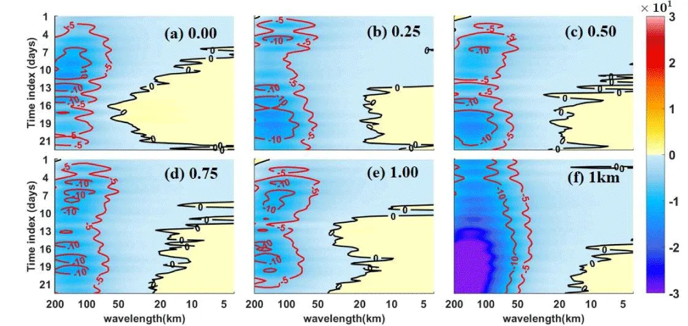
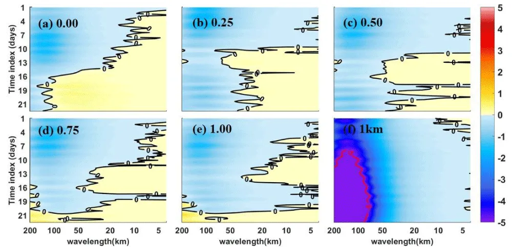
In the submesoscale range below 50 km, the kinetic energy flux exhibits bidirectional characteristics of both forward and upward cascade, but cases with different feedback coefficients show remarkable differences. In the case of a 0.00 feedback coefficient, the flux reveals an overwhelming positive pattern indicative of a forward energy cascade. However, the flux scale range exhibiting positive forward cascade has significantly diminished in cases with 0.25 to 1.00 feedback coefficients. While in the “Truth”, the flux is dominated by negative values associated with inverse cascade across most of the submesoscale scale band, with only a small fraction displaying forward cascades at small wavelengths. This suggests that the scales transitioning from inverse to forward cascades tend to shift to smaller wavelengths when more smaller-scale submesoscales are resolved, consistent with Qiu's study [11], which can also explain that the mesoscales can be strengthened by submesoscale KE to make them more coherent and not quickly dissipated with a KE increase [36].

The scale kinetic energy flux at 200m depth displays similar patterns to those in the upper ocean, despite a significant decrease in intensity. The flux is mainly characterized by inverse cascades across most of the mesoscale range (larger than 50 km). Meanwhile, the flux in the “Truth” is also significantly greater than that of other cases, which confirms that submesoscales can strengthen the mesoscales through inverse kinetic energy cascades even at a depth of 200 m underwater. In the submesoscale range below 50km, the “Truth” shows predominant negative values indicative of inverse cascades, and the scale band associated with inverse cascades has significantly enlarged in cases of 0.25 to 1.00 feedback coefficients compared to that with a 0.00 feedback coefficient. The phenomenon that the scales changing from inverse to forward cascades tend to shift to a smaller wavelength has also been observed.

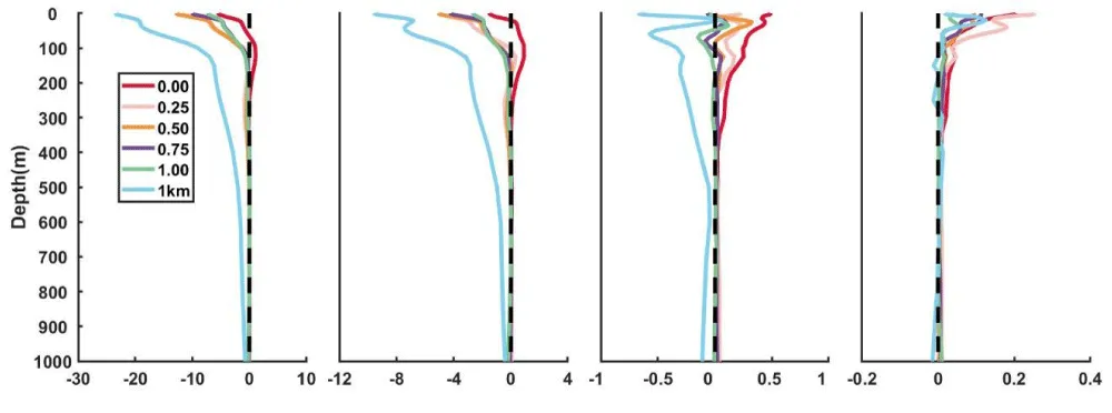
Figure 11 shows the vertical distributions of spatially-averaged scale kinetic energy flux Pl(x) within the upper 1000 m in the feedback area with different feedback coefficients and the “Truth”. Consistent with figure 9 and 10, the inverse kinetic energy cascade is characterized by surface intensification, with the majority concentrated in the larger wavelengths and within the upper 50 meters. However, on a smaller scale, the flux exhibits a weak forward kinetic energy cascade. This energy cascade transition has also been evidenced by Schubert [35] in the Agulhas Current. Specifically, the inverse cascade scale can reach down to about 20 km at the surface in the case of a 0.00 feedback coefficient. However, this scale can further extend to a smaller wavelength of about 8km in cases with 0.25 to 1.00 feedback coefficients, which is very close to the “Truth” whose minimum inverse cascade scale is about 7 km. This suggests that the submesoscale feedback from the finer D2 domain can modify the energy cascade scale, subsequently altering the energy distributions across wavelength space.

Figure 11: Same as Figure 9 but for the vertical distribution of spatial-mean scale Π_l (x).

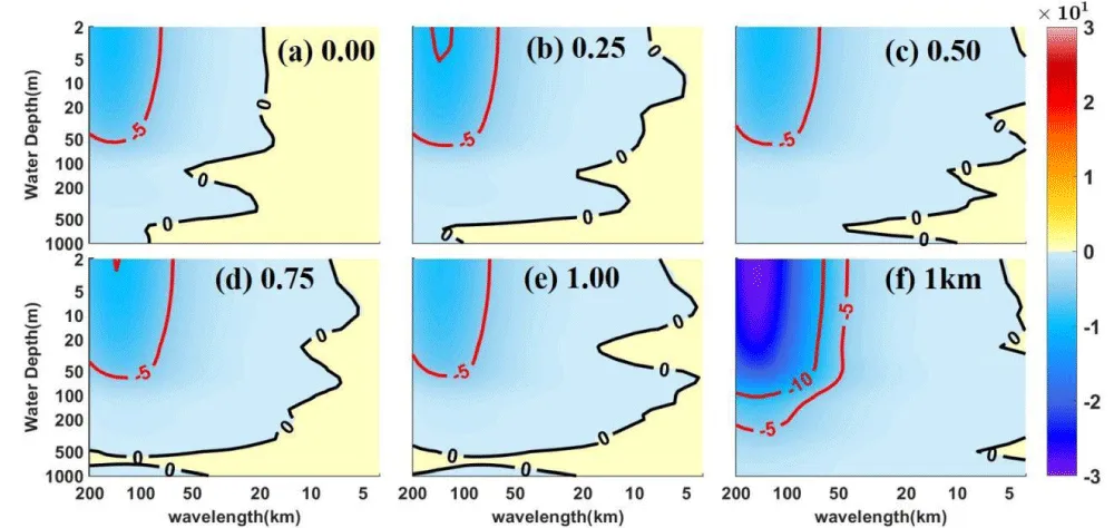
At a depth of 50 m, the scale shifts from inverse to forward cascade transfer below 5 km in the “Truth”, suggesting that there is still a small portion of inverse cascade that has not been resolved by the 1km horizontal resolution. However, in the case of a 0.00 feedback coefficient, this scale remains approximately 20 km, and it is almost unchanged vertically. When the D1 domain acquires refined submesoscale feedback from the D2 domain, this scale significantly decreases to approximately 10 km in cases with feedback coefficients ranging from 0.25 to 1.00. This further validates that the feedback of smaller submesoscales from the D2 1km finer domain can alter the energy cascade transition scale, which would further influence the mesoscales.

Figure 12 shows the time series of surface kinetic energy flux Pl(x) at four different scales of 80 km, 50 km, 15 km, and 5 km in the feedback area from May 20 to June 09, 2018. At larger scales of 80km and 50km, the kinetic energy flux is dominated by negative values associated with inverse cascades [64]. Although the flux in the case with 0.25 to 1.00 feedback coefficients is significantly lower than that in the “Truth”, it has been greatly strengthened by the submesoscale feedback from the finer D2 domain. Meanwhile, the flux is insensitive to the feedback coefficients, which remain at nearly the same level as The feedback coefficients vary from 0.25 to 1.00.

Figure 12: Time series of the surface kinetic energy flux Π_l (x) at four different scales of a) 80 km, b) 50 km, c) 15 km and d) 5 km in the feedback area D2 with different feedback strengths and in the “Truth” from May 20 - June 09, 2018.

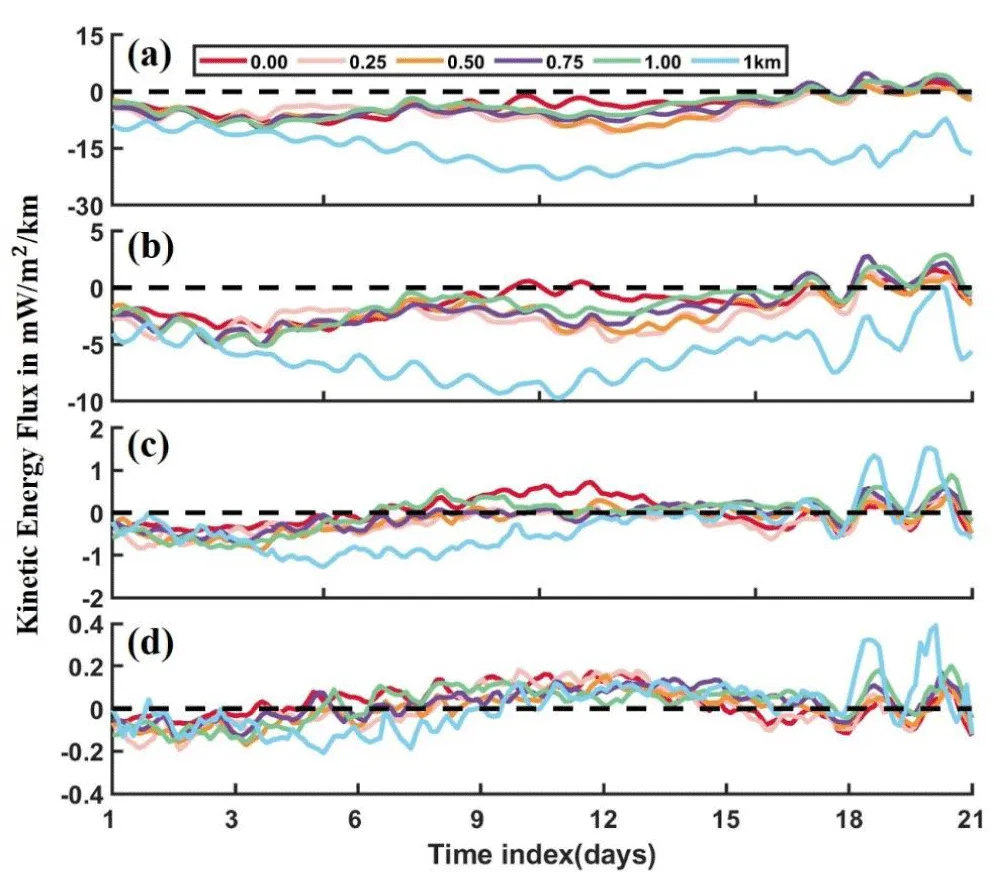
At the smaller scale of 15 km, the flux in the “Truth” remains the inverse cascade most of the time. However, in other cases, the flux gradually transitions from inverse to forward cascades, and the intensity of the forward cascade is strongest in the case with a 0.00 feedback coefficient. This is consistent with a previous study that the change from inverse to forward cascade occurs on smaller wavelengths in the submesoscale permitting model [11,65].

At the D2 domain, with an effective resolution scale of 5 km, almost all surface kinetic energy flux shows negative patterns of forward cascades. Significantly, two peaks of forward cascades appear in the later stages, around 18 to 21 days, among which the magnitude of flux in the “Truth” is the largest, followed by the case with 0.25 to 1.00 feedback coefficients, and the case with 0.00 feedback coefficient shows the smallest value. This may be correlated to the smaller-scale submesoscale processes associated with symmetric instability, which has been recognized as an effective mechanism for forward kinetic energy cascade in the ocean [1,66,67].

In figure 13, we plot the vertical distribution of spatial-mean kinetic energy flux at different scales of 80 km, 50 km, 15 km, and 5 km on June 4, 2018. At the scale of 80km, the kinetic energy flux in all cases shows relatively large negative values indicative of an inverse cascade within the upper ocean, among which the “Truth” is greatly larger than others, and the cases with 0.25 to 1.00 feedback coefficients have been significantly improved compared to that with 0.00 feedback coefficient. Below 100m, the flux in cases with 0.00 to 1.00 feedback coefficients rapidly decreases to 0, while it remains relatively large in the “Truth”. This characteristic is also observed at the 50km scale. The flux in cases of the “Truth” and 0.25 to 1.00 feedback coefficients displays inverse cascade within the upper ocean, although its intensity significantly decreases compared to that at 80km. However, it shows a weak forward cascade in the case with a 0.00 feedback coefficient. At the smaller scale of 15 km, the fluxes show remarkable differences among each other. The “Truth” maintains an inverse cascade throughout the entire water column, but the characteristic of surface intensification is replaced by the sub-surface intensification. The flux in cases with 0.25 to 1.00 feedback coefficients transitions to relatively weak forward cascades within the upper ocean, while in the case with 0.00 feedback coefficient, it behaves as an intense forward cascade. At the D2 domain effective resolution scale of 5 km, all cases show forward cascade within the upper 100m, which indicates the dynamics are dominated by turbulence and dissipation at this scale.

Figure 13: Same as Figure 12 but for the vertical distribution of spatial-mean Π_l (x).

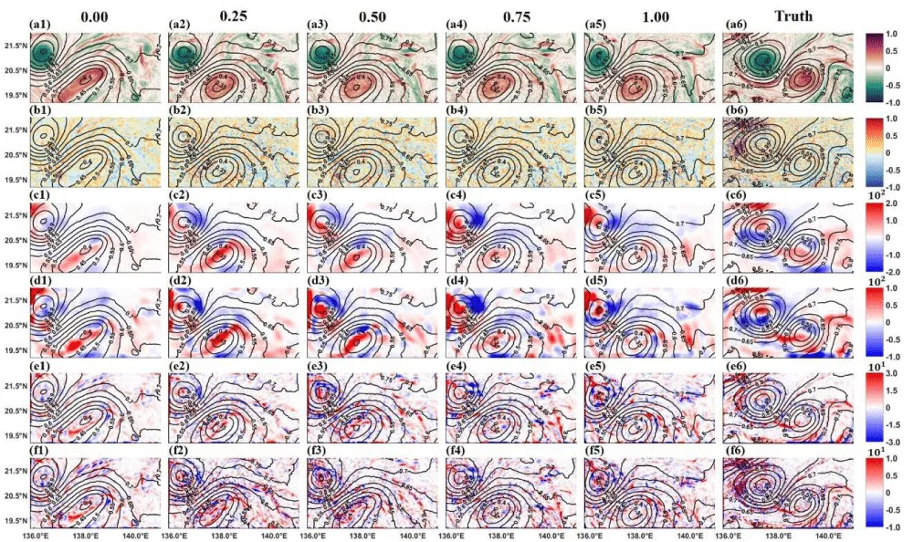
The snapshots of $$\zeta /f$$ , $$Div/f$$ andΠl(x) at four different scales (80 km, 50 km, 15 km, 5 km) with different feedback coefficients and the “Truth” in 10m depth on 20180604 are illustrated in figure 14. As shown in (a1-a6), the cyclonic eddy in mesoscale dipole is severely stretched in case with 0.00 feedback coefficient, while it is more coherent and insensitive to deformation in cases with 0.25 to 1.00 feedback coefficients and the “Truth”. This suggests that when the finer D2 domain provides submesoscale feedback to the coarser D1 domain, this cyclonic eddy is more energetic and not easily dissipated. Moreover, the spatial patterns of $$Div/f$$ (b1-b6) shift toward smaller scales, which is consistent with the conclusion that the peak of $$Div/f$$ tends to shift towards smaller wavelengths as the horizontal resolution increases in the frequency-wavenumber spectra of figure 7. The magnitude of inverse cascades associated with negative kinetic energy flux Πl(x) in scales of 80 km (c1-c6) and 50 km (d1-d6) is increasingly enhanced as the submesoscale feedback increases, which is match to the conclusion in figure 13a and 13b. This also explains that the submesoscales feedback from the D2 domain can strengthen the coherence of the cyclonic eddy in the mesoscale dipole, making it less susceptible to stretching. However, at the smaller scales of 15 km and 5 km, the patterns of Πl(x) in Figure 14 (e1-e6) and (f1-f6) become significantly noisier. Meanwhile, Πl(x) at these scales are gradually dominated by the positive forward cascades instead of inverse cascades, which is consistent with the results in figure 13c and 13d.

Figure 14: The horizontal distribution of surface height anomalies (contours with interval of 0.05 m) with color-shaded a) surface ζ/f, b) surface Div/f and c) 80km scale Π_l (x), d) 50km scale Π_l (x), e) 15km scale Πl (x), and f) 5 km scale Π_l (x) at 10 m depth with different feedback strengths (columns 1-5) and the “Truth” (column 6) on June 04, 2018.

We notice that the kinetic energy levels and scale kinetic energy fluxes are largely insensitive to feedback strength for α ≥ 0.25. It may be related to the limited effective resolution of the D1 domain (3 km). The Mixed-Layer Instability (MLI) typically operates at scales of O (10 km) and serves as a key source of submesoscale kinetic energy, which subsequently drives an inverse energy cascade toward larger mesoscales. In our D1 domain, the 3 km resolution only marginally resolves the MLI scale. As a result, submesoscale processes are significantly under-resolved, leading to an underestimation of submesoscale kinetic energy and, consequently, a weaker inverse cascade. We acknowledge that this resolution limitation may be an important aspect that shall be improved in future studies.

It is worth mentioning that all numerical experiments in this study are conducted using identical topography, lateral boundary conditions, surface forcing, and parameterization schemes, while the feedback coefficient is the only varying factor. Furthermore, the study area is located in the core region of STCC in the northwestern Pacific, which is far from the Kuroshio, so that the influence of strong currents is minimized. In addition, based on previous studies [1,11], a horizontal resolution of 3 (1) km is sufficient to resolve mesoscale (submesoscale) eddies. In that way, our study can focus on the interaction of mesoscales and submesoscales.

A “twin” experiment of two-way nesting with controllable feedback coefficients that can control the feedback strength of submesoscales resolved by a 1 km resolution simulation to the 3 km resolution mesoscale-resolved simulation is designed in this study. A mesoscale dipole of cold-warm eddies appears in the simulation, but the dipole structure does not sustain in the one-way downscaling simulation without submesoscale feedback to mesoscales. When submesoscales provide feedback to the mesoscale eddies, the cyclonic eddy becomes less susceptible to stretching, confirming the significance of submesoscales in regulating mesoscale eddies. Then, the underlying dynamical mechanisms are thoroughly examined from the perspectives of spectral analysis and scale kinetic energy flux in five cases with different feedback strengths. The wavenumber and frequency-wavenumber spectra of Kinetic Energy (KE) reveal a remarkable enhancement when submesoscales provide feedback to the mesoscale eddies, highlighting the importance of submesoscale feedback on mesoscale eddies. Although submesoscales are mainly concentrated within the upper ocean, the frequency-wavenumber spectra of normalized vertical relative vorticity and horizontal divergence are significantly improved at a depth of 200 m. In terms of scale kinetic energy flux, the inverse cascade of KE can extend to smaller scales when submesoscales provide feedback to mesoscale eddies. This indicates that mesoscale eddies can be strengthened when more submesoscales are resolved, further influencing the morphology of the cyclonic eddy in this case. Nevertheless, the energy levels and scale kinetic energy fluxes are insensitive to the feedback strength; both with different feedback strengths exhibit nearly the same magnitudes. Meanwhile, the results indicate a slight increase in forward cascade at a smaller scale, which may be related to the increased dissipation in the grid-resolved scale. The findings in this study can help us to understand the multiscale interactions between mesoscale eddies and submesoscales.

However, we may view this study as the first step on the impact of submesoscale feedbacks on mesoscale activities, and more studies are required in the future to get a complete picture of the impact of submesoscale feedbacks on mesoscale activities. For example, while we demonstrate that increasing model resolution enables explicit resolution of smaller-scale processes at all depths, including 200 m, more analyses on the vertical propagation of submesoscale signals to depths near 200 m can reveal more physics insights. This is because submesoscale dynamics are typically concentrated within the mixed layer; the enhanced vorticity and divergence spectra at depth would further deepen our physical understanding. In our future work, we shall incorporate more quantitative analyses and more numerical experiments to get more systematic conclusions, including consideration of mechanisms such as ageostrophic pumping, buoyancy fluxes, isopycnal slope effects, and internal wave interactions, etc.